The markstat command comes with a help file, so you can type in Stata help markstat. The current version is 2.7, released June 2nd, 2021.
The basic idea is very simple. You type a script that contains a narrative written in Markdown, and include Stata code that is indented one tab or four spaces, as in the following example
Let's read the fuel efficiency data that comes with Stata,
compute gallons per 100 miles, and regress that on weight

    sysuse auto, clear
    gen gphm = 100/mpg
    regress gphm weight

We see that heavier cars use more fuel, with 1,000 pounds requiring
an extra 1.4 gallons to travel 100 miles
This simple rule is all it takes. The markstat command will read this script and generate a web page, PDF file or Word document that combines the code with the output and your narrative. (Or even a slide show, as described below.) Here’s the HTML output:
Let’s read the fuel efficiency data that comes with Stata, compute gallons per 100 miles, and regress that on weight
. sysuse auto, clear
(1978 automobile data)

. gen gphm = 100/mpg

. regress gphm weight

      Source │       SS           df       MS      Number of obs   =        74
─────────────┼──────────────────────────────────   F(1, 72)        =    194.71
       Model │  87.2964969         1  87.2964969   Prob > F        =    0.0000
    Residual │  32.2797639        72  .448330054   R-squared       =    0.7300
─────────────┼──────────────────────────────────   Adj R-squared   =    0.7263
       Total │  119.576261        73  1.63803097   Root MSE        =    .66957

─────────────┬────────────────────────────────────────────────────────────────
        gphm │ Coefficient  Std. err.      t    P>|t|     [95% conf. interval]
─────────────┼────────────────────────────────────────────────────────────────
      weight │    .001407   .0001008    13.95   0.000      .001206    .0016081
       _cons │   .7707669   .3142571     2.45   0.017     .1443069    1.397227
─────────────┴────────────────────────────────────────────────────────────────
We see that heavier cars use more fuel, with 1,000 pounds requiring an extra 1.4 gallons to travel 100 miles.
The command goes through the script and separates the Markdown narrative, which goes in a .md file with all Stata code removed, and the Stata code, which goes in a .do file with all annotations removed. We call this the tangle step.
The .md file is just plain Markdown. We use a placeholder of the form {{n}}, where n is a chunk number, to mark where the Stata code block used to be, so please don’t use double braces in your narrative.
The .do file is just plain Stata. We insert a comment of the form //_n to mark the beginning of the n-th code chunk, and //_^ to mark the end of the last chunk, so please avoid these patterns if you include comments. The command runs this file through Stata to obtain a .smcl log.
The next step is to weave together the Markdown and Stata output, using the information in the placeholders and markers to know where everything goes. The exact sequence of steps depends on the output format, but is transparent to you.
We rely on Pandoc to translate Markdown to HTML or LaTeX and to generate a Word document. To produce PDF output via LaTeX the command will then run a LaTeX-to-PDF converter. See the Getting Started section for installation help.
The script file may be edited using Stata’s code editor, which has the advantage that you can select and run your Stata code to check that it works, or to examine results while you are authoring the narrative.
The syntax of the command is as follows
markstat using filename [, pdf docx slides beamer mathjax
    bundle bibliography strict nodo nor keep ]
The only required argument is the name of the script file. This must have extension .stmd, but the extension does not have to be typed. I highly recommend that you run Stata from the same directory where you stored the script.
If you are producing HTML and do not have complex mathematical equations, you don’t need any of the options, so let me give you just a brief summary here:
pdf is used if you want to generate a PDF document, which we do via LaTeX, so this option requires additional tooling as explained in Getting Started.
docx is used to generate a Word document instead. Just like that!
slides generates an HTML slide show using the S5 engine and the default Blue Spiral theme, and slides(santiago) uses the Santiago theme. Add a + for incremental mode, typing slides(+) or slides(santiago+).
beamer generates a PDF slide show via LaTeX using Beamer and the default theme, and beamer(theme) uses any of the many Beamer themes available, for example beamer(madrid). Add a + for incremental mode.
mathjax is use to activate the MathJax JavaScript library, which does an excellent job of rendering mathematical equations on the web. Not needed for PDF or Word documents, where LaTeX equations are rendered natively.
bundle is used to generate self-contained HTML documents, encoding all images and ancillary files using base64. MathJax cannot be bundled, but a local link is used instead. This option is not needed for PDF or Word documents, which are always self-contained.
bibliography is used to resolve citations using a BibTeX database and generate a list of references at the end of the document, as explained below. Works with all formats.
strict controls the way the command distinguishes Markdown annotations from Stata commands, as explained in the Stata code section below. Code fences are now detected automatically, so this option can be omitted in most cases.
nodo is used to skip running the Stata code when you have just tweaked the narrative. Useful for presentations, where you may change from S5 to Beamer, or try a different theme, without rerunning the analysis. The idea comes from Ben Jann’s nodo option in texdoc.
nor is the equivalent of nodo for R code, and will skip running R commands, using instead the most recent output.
keep will save intermediate files which are now deleted to avoid cluttering your hard drive. By default we keep only smcl and rout files to enable nodo and nor, in addition of course to the output files. Use keep to keep everything and keep(list) to keep selected files, for example keep(do R) to keep the generated Stata do file and R script.
Markdown is a lightweight markup language invented by John Gruber. It is easy to write and, more importantly, it was designed to be readable “as is”, without intrusive markings.
Gruber’s Markdown: Basics has a quick introduction to the notation. There is an ongoing effort to standardize Common Markdown with reference implementations in C and JavaScript, see commonmark.org for details.
The markstat command uses John MacFarlane’s Pandoc to
convert Markdown to HTML or LaTeX, so you first need to install this converter
as explained in Getting Started.
In Markdown you create a heading by “underlining” the title with === for level 1 and --- for level 2. You can also define a heading at levels one to six by starting a line with one to six hashmarks, as in ### A level 3 heading.
You define a paragraph break by leaving a blank line. If you need a line break leave two or more spaces at the end of the line, or end the line with a backslash \, a Pandoc extension that makes the line break clearer.
To indicate emphasis using italics wrap the text using an asterisk or underscore, as in *italics*. For strong emphasis using a bold font wrap the text using two asterisks or underscores, as in **bold**. For a monospace font suitable for code use backticks, for example to refer to the regress command type regress.
To create a list you start a line with an asterisk *, plus +, or minus - sign for a bulleted list, or a number followed by a period, for example 1., for a numbered list. You add items to a list by starting a line with the same symbol or with a number. Items in ordered lists are numbered consecutively starting with the first number, regardeless of the numbers actually used for the other items. To end the list enter a blank line.
You can link to another document by putting the anchor in square brackets and the link in parentheses, as in [Markstat's website](https://grodri.github.io/markstat) to link to this website.
To link to an image start with a bang, type a title in square brackets and the source in parentheses, as in 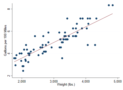.
Markdown lets you include HTML as well, so we could have coded the image as <img src='auto.png' alt='Fuel Efficiency'/> and a line break as <br/>. This is not recommended if the aim is to generate documents in other formats.
Pandoc interprets any text between dollar signs as a LaTeX formula, so you may write a regression equation as $y = \alpha + beta x + e$. If you are generating HTML this will be rendered by default using Unicode characters. For best results, however, use the mathjax option to link to the MathJax JavaScript library, which does a an excellent job rendering LaTeX equations. If you are rendering PDF via LaTeX the equations are rendered natively by LaTeX. If you are generating a docx file, Pandoc translates LaTeX to native Word equation objects.
In addition to inline equations you can include displayed equations by using double dollar signs as in the following example
$$
    y = \alpha + \beta x + e
$$
I think indenting the equation as above improves readability, and markstat ensures that equations in display blocks are not confused with Stata code.
Pandoc allows including the document’s title, author and date as metadata; just
start the document with three lines that begin with % and contain this information:
% Stata Markdown
% Germán Rodríguez
% 26 October 2016
If you want to use the date when the document was run, you can type
`s c(current_date)` instead of an explicit date.
Inline code is explained below.
Alternatively, you may use the YAML format, a block starting and ending with
three dashes ---:
---
title: Stata Markdown
author: Germán Rodríguez
date: 26 October 2016
---
Here you can also use inline code for the date, just include it in quotes to keep YAML
happy, so the last line would be date: "`s c(current_date)`".
An important advantage of the YAML format is that it allows us to include other
information for Pandoc, for example the name of a bibliography file used to resolve citations as explained here, or an abstract to be used in PDF documents
via LaTeX. For an example using both features, see the metadata for the original markstat paper here.
Pandoc 2.0 and higher requires HTML documents to have a title, and issues a warning if the title is missing.
The simple “one tab or four spaces” rule to distinguish Stata and Markdown code works well, but precludes some advanced Markdown options such as nested lists.
The strict option of markstat uses code fences instead, with Stata code blocks defined as
```s
  // Stata code goes here
```
The s may be enclosed in braces if you wish, so the opening fence may be coded
```{s}.
You can supress echoing the commands in a Stata block using the syntax
```s/
  // Commands here are not echoed
```
The opening fence may also be ```{s/}. Of course you can always supress output using quietly.
Code inside fences may be indented to improve readability. The markstat command will remove one level of indentation if present.
A Stata block can always enter Mata using mata: and exit using end, but you can also code a Mata block directly using an m instead of an s. For an example see Mata Matters.
You can also include R code in fenced blocks using an r instead of an s, provided of course you have R installed. For an example see quantiles in Stata and R.
If markstat detects use of Stata, Mata or R fenced code blocks in the first 50 lines of your script, it will set strict mode automatically, so you can omit that option in most cases.
You can quote results by including inline code as part of your narrative, using the syntax `s [fmt] expression`, where fmt is an optional format, followed by an expression.
The markstat command will generate code to evaluate the expression using Stata’s display command, and will splice the output inline with the text.
For example after running a regression you can cite R-squared by coding
`s e(r2)`. If you prefer to display the value with 2 decimal places only,
use `s %5.2f e(r2)`.
Consistent with our treatment of Mata as a first class citizen, you can also include inline Mata code using the same syntax, but with an m instead of an s. The markstat command will generate a printf() function call to display the expression with the given format. If the format is omitted it defaults to %s, so the expression should yield a string.
You can also quote R results using inline code with the syntax
`r expression`. There is no optional format, but you can always use R’s round(). For examples see quantiles.
Markdown does not have a syntax for tables, but Pandoc provides a simple syntax, best explained through an example. The code below shows average fuel efficiency in gallons per 100 miles for foreign and domestic cars before and after adjusting for weight:
Car Type    Unadjusted   Adjusted
--------- ------------ ----------
Foreign        4.31         5.46
Domestic       5.32         4.83
Basically you type the column headers, some underlining, and then the table lining up the columns yourself. The cell alignment is determining by the position of the header relative to the underlining. Our first column is left aligned and the other two are right aligned.
Unfortunately this syntax will not work with inline code because the expressions, the placeholders and the final output may all have different widths. Fortunately Pandoc has an alternative syntax using pipe tables, where columns are separated by the pipe character |, and alignment is indicated by placing a colon in the header underlining. The previous table would be coded as follows:
| Car Type | Unadjusted |  Adjusted|
|:---------|-----------:|---------:|
| Foreign  |   4.31     |   5.46   |
| Domestic |   5.32     |   4.83   |
I lined up the pipe characters for readability, but this is not required. Both tables render the same way.
Combining inline code with pipe tables lets us produce dynamic reports. An example generating the above table from scratch may be found here.
Another example generating a table of estimates using Jann’s esttab command may be found here.
Figures are rendered by default using their actual size in HTML and 75% of the line width in PDF via LaTeX, but you can tinker with the size. Specifically, you can add a width attribute to the Markdown link, specifying a width in inches using in, in centimeters using cm, or a relative size using %, as in the following example
{width=100%}
which sets the width of the image to the full page width (minus the margins). Here are some practical recommendations.
For HTML I typically use PNG images with a width of 500 pixels, which at 96 dots per inch makes them just over 5 inches wide. The physical size is set with the width option of Stata’s graph export command. I then render them at their natural size using a default link. If I specified a relative width of 100% the image would grow and shrink as the browser resizes.
For PDF the best results are obtained if the graph is saved in PDF format, as this contains instructions to draw the image at any desired resolution, including 300 dpi for printers. By default the graph is included in LaTeX at 75% of the line width, but you can change the percentage as noted above. It is also possible to use a PNG image, which in my experience looks good enough if the image is at least 500 pixels wide.
Thanks to the amazing Pandoc, markstat can also handle bibliographic references.
In a nutshell, you create a BibTeX database with the literature you intend to cite, and include a reference to that file in the documents YAML metadata.
Each reference has a unique key, for example knuth92, and you can cite it in the text using an ampersand and the key, as in @knuth92, with options to include page numbers and other information.
Using the bibliography option coordinates with Pandoc’s cite-proc to resolve the references and list them at the end of the document. More information
here.
Thanks also to Pandoc, markstat provides a user-friendly interface for producing slide shows in HTML using the S5 engine or in PDF format using Beamer, using plain Stata code combined with a narrative written in Markdown with a few simple conventions.
A slide show using S5 or Beamer must start with a metadata block providing the title, author and date of the presentation. This information is used to produce a title slide. This is followed by Stata and Markdown code using the simple or strict syntax to define each slide.
In a simple presentation, each heading at level 1 defines a slide and is followed by contents, usually bullet points, and figures and tables generated using Stata. In a multipart presentation, level-1 headings define parts and generate title slides, and level-2 headings define slides. Pandoc figures out the slide level looking for the highest level heading followed immediately by contents.
When you create a presentation you include figures using the Markdown syntax {width="60%"}. I recommend that you always specify a relative size as shown in this example. If you are using Beamer, add {.fragile} to the heading of slides that contain Stata commands or output (or any verbatim content).
An introductory example using the simple syntax is found here. Another example using the strict syntax and taking advantage of Pandoc newly-added syntax for columns is found here.
Numbering and cross-referencing of chapters, sections, tables, figures and equations is still work in progress. Users generating PDF via LaTeX, may rely on native LaTeX features, as shown in this example.
Updated for markstat 2.3