
We conclude our competing risk analysis of supreme court tenure by fitting the Fine and Gray model, which focuses on the sub-hazard of each risk.
We use the file saved earlier, see. Alternatively, you may rebuild the dataset using the first block of code in that page.
We read the data and recode dates as before. (You can skip this step if you are runing this code in the same session as the previous page.)
. use https://grodri.github.io/datasets//justices2, clear
> justices <- read.csv("https://grodri.github.io/datasets//justices2.csv")
This model can be fit in Stata using the
stcrreg command, with death as the event of interest as
retirement as the competing event. We fit the
model using the crr function in the cmprsk
package. The function requires a model matrix instead of a model
formula. In our example the matrix is simple, for more general help type
?model.matrix. I specify the codes for the event of
interest and for censoring, although they happen to coincide with the
defaults.
. stset tenure, fail(event == 1)

Survival-time data settings

         Failure event: event==1
Observed time interval: (0, tenure]
     Exit on or before: failure

──────────────────────────────────────────────────────────────────────────
        113  total observations
          0  exclusions
──────────────────────────────────────────────────────────────────────────
        113  observations remaining, representing
         50  failures in single-record/single-failure data
  1,887.365  total analysis time at risk and under observation
                                                At risk from t =         0
                                     Earliest observed entry t =         0
                                          Last observed exit t =  36.57221

. stcrreg age year, compete (event == 2)

        Failure _d: event==1
  Analysis time _t: tenure

Iteration 0:   log pseudolikelihood =  -216.0489
Iteration 1:   log pseudolikelihood = -211.97443
Iteration 2:   log pseudolikelihood = -211.87323
Iteration 3:   log pseudolikelihood = -211.87319
Iteration 4:   log pseudolikelihood = -211.87319

Competing-risks regression                        No. of obs      =        113
                                                  No. of subjects =        113
Failure event:   event == 1                       No. failed      =         50
Competing event: event == 2                       No. competing   =         54
                                                  No. censored    =          9

                                                  Wald chi2(2)    =      14.84
Log pseudolikelihood = -211.87319                 Prob > chi2     =     0.0006

─────────────┬────────────────────────────────────────────────────────────────
             │               Robust
          _t │        SHR   std. err.      z    P>|z|     [95% conf. interval]
─────────────┼────────────────────────────────────────────────────────────────
         age │   1.007446   .0176847     0.42   0.673     .9733737     1.04271
        year │   .9915572   .0023216    -3.62   0.000     .9870173     .996118
─────────────┴────────────────────────────────────────────────────────────────
> library(cmprsk)
> fg <- crr(justices$tenure, justices$event, justices[,c("age", "year")],
+     failcode = 1, cencode = 0)
> summary(fg)
Competing Risks Regression

Call:
crr(ftime = justices$tenure, fstatus = justices$event, cov1 = justices[,
    c("age", "year")], failcode = 1, cencode = 0)

         coef exp(coef) se(coef)      z p-value
age   0.00742     1.007  0.01748  0.424 0.67000
year -0.00848     0.992  0.00233 -3.637 0.00028

     exp(coef) exp(-coef)  2.5% 97.5%
age      1.007      0.993 0.974 1.043
year     0.992      1.009 0.987 0.996

Num. cases = 113
Pseudo Log-likelihood = -212
Pseudo likelihood ratio test = 13.2  on 2 df,
We see that the probability that a judge will die while in the court doesn’t appear to vary with age at appointment, but decreases with calendar year of appointment, so judges appointed more recently are less likely to die while serving in the court.
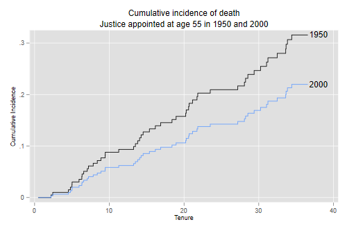
We predict the CIF of death for a justice appointed at age 55 completed years in 1950 and 2000. The code below adds 0.5 to convert to exact ages and mid years.)
. stcurve, cif at1(age = 55.5 year = 1950.5) at2(age = 55.5 year = 2000.5) ///
>     title("Cumulative incidence of death") xtitle(Tenure) ///
>     subtitle("Justice appointed at age 55 in 1950 and 2000") ///
>     text(.22 38 "2000") text(.316 38 "1950") legend(off)

. graph export justices-ciffg.png, width(500) replace
file justices-ciffg.png saved as PNG format
Aside: It is instructive to compute
these curves ‘by hand’. Because predict sets the covariates
to zero, it will be advantageous to center age on 55.5 and year on
1950.5, as we did for the Cox model, so the predicted survival is our
first scenario.
. gen agec = age - 55.5

. gen yearc = year - 1950.5

. quietly stcrreg agec yearc, compete(event==2)

. predict cif1950, basecif
We know that this model is linear in the c-log-log scale, so we transform the CIF for 1950, add 50 times the year coefficient, and then transform back to probabilities.
. gen cif2000 = invcloglog( cloglog(cif1950) + 50 * _b[yearc] )
(4 missing values generated)

. sort _t

. twoway line cif1950 _t, c(J) || line cif2000 _t, c(J) legend(off)

. list _t cif1950 cif2000 in -1

     ┌─────────────────────────────────┐
     │        _t    cif1950    cif2000 │
     ├─────────────────────────────────┤
113. │ 36.572212   .3156297   .2198049 │
     └─────────────────────────────────┘
> nd <- matrix(c(55.5, 55.5, 1950.5, 2000.5), 2, 2)
> cifs <- predict(fg, nd)
> cifd <- data.frame(
+     year = factor(rep(c("1950", "2000"), rep(nrow(cifs),2))),
+     time = c(cifs[,1], cifs[,1]),
+     cif = c(cifs[,2], cifs[,3])
+ )
> library(ggplot2)
> ggplot(cifd, aes(time, cif, color=year)) + geom_step()
> ggsave("justices-ciffgr.png", width = 500/72, height = 400/72, dpi = 72)
> cifs[nrow(cifs),]
[1] 34.4147844  0.3156297  0.2198049
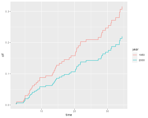
We see that the probability of dying while serving in the court is declining over time net of age at appointment. For a justice appointed at age 55, the probability would be 31.6% if appointed in 1950 and 22.0% if appointed in the year 2000, assuming of course that current trends continue, so the model applies.
Incidence functions can also be computed from Cox models, which in my view have a clearer interpretation, as shown here. The Cox proportional hazards approach leads to estimated probabilities of death of 32.8% if appointed in 1950 and 22.6% if appointed in 2000. Both methods agree in estimating the overall decline as about ten percentage points.