
Singer and Willet (2003) Applied Longitudinal Data Analysis, Oxford, analyze data on the length of service of U.S. Supreme Court Justices, treating death and retirement as competing risks, and age at appointment and calendar year of appointment as predictors.
To conduct a similar analysis I extracted data from Wikipedia and the Supreme Court website, and prepared a comma-separated-value file with the justice number, name, and strings representing the dates of birth, the dates tenure starts and stops, and a status variable that takes the values Incumbent, Died, Resigned or Retired. I ignore the return engagements of John Rutledge and Charles Evans Hughes, who resigned and later were reappointed as Chief Justice.
The file is available on this website as justices.csv
and can be read as shown in the Stata and R logs. All dates include the
day, month and year. The date of birth of James Moore Wayne was
available as year only in both sources, so I set the month and day to
July 1. All other dates were complete. (An earlier version of this
dataset recorded all dates using years only, for simplicity and
consistency with the reference. That version is available in Stata 11
format as justices.dta. It was last updated in 2016.)
We start by reading the data and converting the dates from strings to
the native date format in your statistical package. Note that
stopstr is empty for incumbents. We set it to February 22,
2018 for these cases, effectively censoring the data as of the date this
analysis was run. I calculate tenure in years dividing by
365.25. The event indicator is coded 0 for current
Justices, 1 for those who died while serving, and 2 for those who
resigned or retired. I also compute age at appointment and
year of appointment, and save the dataset for later
use.
. import delimited using https://grodri.github.io/datasets/justices.csv, clear
(encoding automatically selected: ISO-8859-1)
(7 vars, 113 obs)

. gen birth = date(birthstr, "MDY")

. gen start = date(startstr, "MDY")

. replace stopstr = "February 22, 2018" if stopstr == ""
(9 real changes made)

. gen stop = date(stopstr, "MDY")

. gen tenure = (stop - start)/365.25

. gen event = (status == "Died") + ///
>     2*(status == "Resigned" | status == "Retired")

. gen age = (start - birth)/365.25

. gen year = year(start) + (doy(start)-1)/doy(mdy(12,31,year(start)))

. drop *str

. save justices2, replace
file justices2.dta saved
> justices <- read.csv("https://grodri.github.io/datasets/justices.csv",
+     stringsAsFactors = FALSE)
> table(justices$status)

     Died Incumbent  Resigned   Retired
       50         9        17        37
> library(dplyr)
> library(lubridate)
> map <- data.frame(code=c(0,1,2,2))
> row.names(map) <- c("Incumbent","Died","Resigned","Retired")
> justices <- mutate(justices,
+     birth = mdy(birthstr),
+     start = mdy(startstr),
+     stop  = mdy(ifelse(stopstr=="", "February 22, 2018", stopstr)),
+     tenure = (stop - start)/365.25,
+     event = map[status,],
+     age  = (start - birth)/365.25,
+     year = year(start) +
+         (yday(start)-1)/ifelse(leap_year(year(start)),366,365)) |>
+ select(-ends_with("str"))
> write.csv(justices, file = "justices2.csv")
The first thing we calculate is the Kaplan-Meier estimator of overall survival
. stset tenure, fail(event) // event > 0

Survival-time data settings

         Failure event: event!=0 & event<.
Observed time interval: (0, tenure]
     Exit on or before: failure

──────────────────────────────────────────────────────────────────────────
        113  total observations
          0  exclusions
──────────────────────────────────────────────────────────────────────────
        113  observations remaining, representing
        104  failures in single-record/single-failure data
  1,887.365  total analysis time at risk and under observation
                                                At risk from t =         0
                                     Earliest observed entry t =         0
                                          Last observed exit t =  36.57221

. sts graph

        Failure _d: event
  Analysis time _t: tenure

. graph export justices-km.png, width(500) replace
file justices-km.png saved as PNG format

. sts gen km = s // save for later use

. list _t km if abs(km - 0.5) < 0.01

     ┌───────────────────────┐
     │        _t          km │
     ├───────────────────────┤
 15. │ 16.156057   .50834001 │
 89. │ 16.490076    .4989263 │
     └───────────────────────┘
> library(survival)
> km <- survfit(Surv(tenure, event > 0) ~ 1, data=justices)
> km
Call: survfit(formula = Surv(tenure, event > 0) ~ 1, data = justices)

       n events median 0.95LCL 0.95UCL
[1,] 113    104   16.5    14.3    20.3
> source("ggfy.R.txt")
> png("justices-kmr.png", width=500, height=400)
> ggfy(km)
> dev.off()
null device
          1
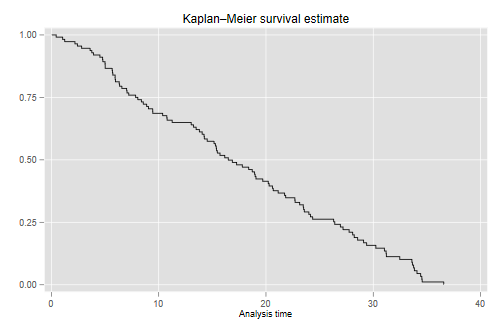
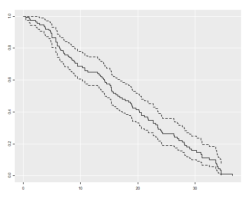
The median length of tenure in the court is 16.5 years.
We will use the command stcompet,
written by V. Coviello and M. Boggess (2004) “Cumulative incidence
estimation in the presence of competing risks” Stata Journal,
4(2):103-112, to estimate incidence functions. We specify death as the
event of interest and retirement as the competing event. We will use the function cuminc() in Bob Grays’s
cmprsk package to estimate cumulative incidence
functions.
. streset, fail(event == 1)
-> stset tenure, failure(event==1)

Survival-time data settings

         Failure event: event==1
Observed time interval: (0, tenure]
     Exit on or before: failure

──────────────────────────────────────────────────────────────────────────
        113  total observations
          0  exclusions
──────────────────────────────────────────────────────────────────────────
        113  observations remaining, representing
         50  failures in single-record/single-failure data
  1,887.365  total analysis time at risk and under observation
                                                At risk from t =         0
                                     Earliest observed entry t =         0
                                          Last observed exit t =  36.57221

. stcompet ci = ci, compet(2) // you just specify the code
> library(cmprsk)
> cif <- cuminc(justices$tenure, justices$event)
> cifd <- data.frame(
+     cause = factor(rep(c("death","retirement"),
+             c(length(cif[[1]]$time), length(cif[[2]]$time)))),
+     time  = c(cif[[1]]$time, cif[[2]]$time),
+     cif   = c(cif[[1]]$est,  cif[[2]]$est))
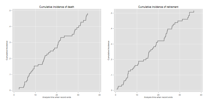
The code generates the cumulative incidence functions CIF for each
competing cause. To plot them you need to select the
appropriate event code. I stacked them into a
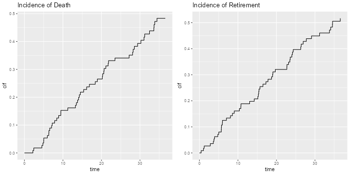
data frame suitable for use with ggplot(). Here’s
the incidence of death and retirement
. twoway line ci _t if event==1, c(J) sort ///
>     title(Cumulative incidence of death) name(d, replace)

. twoway line ci _t if event==2 & _t > 0, c(J) sort ///
>     title(Cumulative incidence of retirement) name(r, replace)

. graph combine d r, xsize(6) ysize(3)

. graph export justices-cif.png, width(720) height(360) replace
file justices-cif.png saved as PNG format
> library(ggplot2)
> g1 <- ggplot(filter(cifd, cause=="death"), aes(time, cif)) +
+     geom_step() + ggtitle("Incidence of Death")
> g2 <- ggplot(filter(cifd, cause=="retirement"), aes(time, cif)) +
+     geom_step() + ggtitle("Incidence of Retirement")
> library(gridExtra)
> g <- arrangeGrob(g1, g2, ncol=2); #plot(g)
> ggsave(plot = g, "justices-cifr.png", width = 10, height = 5, dpi = 72)
We now build a nice plot that combines the Kaplan-Meier estimate of overall attrition with the cumulative incidence functions showing atrition by cause. This takes a bit of work, but I think the result is worth the effort.
We use the fact that the survival and incidence functions add up to one, S(t) + I1(t) + I2(t) = 1, so the areas in the plot have boundaries 1, 1 - I1(t), S(t) and 0. The survival can be obtained from Kaplan-Meier or as the complement of the sum of the incidence functions.
In Stata we start by extracting the CIF for death, and fill in the times for other types of events, which are coded as missing. We also add a dummy observation so the plot actually starts at time 0.
. sort _t

. gen cid = ci if event==1
(63 missing values generated)

. replace cid = cid[_n-1] if missing(cid)
(59 real changes made)

. replace cid = 0 if missing(cid)
(4 real changes made)

. expand 2 in -1 // new observation is at the end
(1 observation created)

. replace _d = . in -1
(1 real change made, 1 to missing)

. replace _t = 0 in -1
(1 real change made)

. replace km = 1 in -1
(1 real change made)

. replace cid = 0 in -1
(1 real change made)

. // We can now compute the boundaries and plot them
. gen b1 = 1

. gen b2 = 1 - cid

. gen b3 = km

. gen b4 = 0

. sort _t

. twoway rarea b1 b2 _t, color("255 160 160") c(J) ///
> ||  rarea b2 b3 _t, color("160 160 255") c(J) ///
> ||  rarea b3 b4 _t, color("160 255 160") c(J) ///
> , legend(off)  xtitle(Years) text(.2 15 "Active") ///
>   text(.5 25 "Retired") text(.8 30 "Died") ///
>   title("Status of Justices by Years since Appointment") ///
>   plotregion(color(white)) graphregion(color(white))

. graph export justices-status.png, width(600) replace
file justices-status.png saved as PNG format

. drop in 1 //remove dummmy
(1 observation deleted)
In R we have to deal with the fact that
survfit() and cuminc() arrange their results
differently, and that the times do not line up. My solution merges the
estimates and uses a simple function to fill the gaps. For the plot
itself I found it easier to draw the areas using
polygon().
> # align times and fill gaps
> death <- filter(cifd, cause=="death");
> retirement <- filter(cifd, cause=="retirement")
> dr <- full_join(death, retirement, by = "time") |>
+     select(time, death=3, retirement=5) |> arrange(time)
> fg <- function(x) {
+     for(i in 2:length(x)){
+         if(is.na(x[i])) x[i] <- x[i-1]
+     }
+     x
+ }
> dr <- mutate(dr, death = fg(death), retirement = fg(retirement))
>
> # draw the graph using overlapping polygons
> png("justices-statusr.png", width=600, height=500)
> par(mar=c(2,2,1,1), mgp=c(2 ,.7, 0), tck=-.01, cex=0.75)
> tmax = max(dr$time)
> plot(c(0, tmax), c(0,1), type="n", xlab="time", ylab="survival")
> polygon(c(0,tmax,tmax,0), c(0,0,1,1),
+     col="#FFA0A0", border="#FFA0A0")
> text(30, .8, "Died")
> polygon(c(dr$time,tmax,0),c(1 - dr$death, 0, 0),
+     col = "#A0A0FF", border = "#A0A0FF")
> text(25, .5, "Retired")
> polygon(c(dr$time,tmax,0),c(1 - dr$death - dr$retirement, 0, 0),
+     col="#A0FFA0", border ="#A0FFA0")
> text(15, .2, "Active")
> dev.off()
pdf
  2
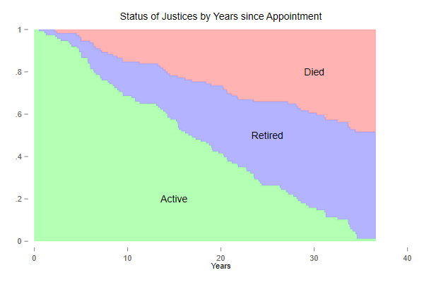
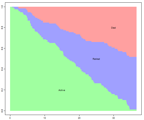
The green area is the survival function, showing the probability of remaining in the court, and the other two areas partition attrition into death and retirement, based on the incidence functions. In the long run death and retirement are approximately equally likely.