
We illustrate the analysis of repeated measurements following the example in Chapter 10 of the MLwiN manual, involving the results of reading tests for a cohort of students in 33 infant schools in the UK. The students entered in 1982 and were measured annually from 1982 to 1986 and again in 1989. Different tests were used at different ages, and the response was standardized to have a mean that increases linearly with age and has a constant coefficient of variation.
The data are on wide format, with each reading score (and age) on a separate variable. Missing data are coded as -10. The first task is to convert the dataset to long format. You may want to do this sort of manipulation in Stata. We will use MLwiN. You can follow the instructions in the manual using the GUI or try the following commands (with explanatory notes). Make sure you substitute the location of MLwiN on your computer.
retrieve c:\program files\mlwin1.10\reading1.ws
note define -10 as missing value code
miss -10
note repeat each id six times in c17
repe 6 "id" c17
note stack all six reading scores in c14 (indicator in c16)
vect 6 "read1" "read2" "read3" "read4" "read5" "read6" c14 c16
note stack all six ages in c15 (indicator in c16)
vect 6 "age1" "age2" "age3" "age4" "age5" "age6" c15 c16
put 2442 1 c18
name c14 "reading" c15 "age" c16 "occassion" c17 "student" c18 "one"The first analysis in the manual is a simple variance-components model
respon "reading"
ident 1 "occassion" 2 "student"
note a variance components model
expla 1 "one"
setv 1 "one"
setv 2 "one"
batch 1
start
fixed
random
The output shown below indicates that most of the variation is within students across occassions, but we haven’t allowed for growth yet.
Convergence achieved
fixed


  PARAMETER            ESTIMATE     S. ERROR(U)   PREV. ESTIMATE
one                       7.115      0.05303              7.115
random
LEV.  PARAMETER       (NCONV)    ESTIMATE    S. ERROR(U)  PREV. ESTIM     CORR.
-------------------------------------------------------------------------------
 2    one      /one      ( 1)     0.07761        0.08309      0.07723         1
-------------------------------------------------------------------------------
 1    one      /one      ( 2)       4.562         0.1725        4.562
like
977608 spaces left on worksheet

-2*log(lh) is 7685.74Next we introduce age. If you fit age as a fixed effect you will see that the coefficient is very close to one (0.997), which is not surprising because this is how the outcome was standardized. We will treat age as random at level 2 so each student can have his or her own slope. Because the use of constant coefficient of variation causes the variance to increase with age we also make age random at level 1. This allows the variance to be a quadratic function of age, which is just what we want.
note a linear growth curve model
expla 1 "age"
setv 1 "age"
setv 2 "age"
start
fixed
random
like
And here are the results:
convergence achieved
fixed


  PARAMETER            ESTIMATE     S. ERROR(U)   PREV. ESTIMATE
one                       7.117       0.0439              7.117
age                       0.995      0.01232              0.995
random
LEV.  PARAMETER       (NCONV)    ESTIMATE    S. ERROR(U)  PREV. ESTIM     CORR.
-------------------------------------------------------------------------------
 2    one      /one      ( 2)      0.7048        0.05433       0.7043         1
 2    age      /one      ( 2)      0.1279        0.01276       0.1278     0.809
 2    age      /age      ( 2)     0.03545       0.004031      0.03537         1
-------------------------------------------------------------------------------
 1    one      /one      ( 2)      0.1227       0.008259       0.1228
 1    age      /one      ( 1)   0.0006868        0.00273    0.0006908
 1    age      /age      ( 1)      0.0145       0.003046       0.0145
like
977583 spaces left on worksheet

-2*log(lh) is         3177
We see substantial variation around the average slope of one. If you fit the new terms in this model one at a time you will see that the deviance statistic (-2logL) is reduced as follows
| Age | -2logL |
|---|---|
| not included | 7685.736 |
| fixed | 3795.589 |
| random at level 2 | 3209.392 |
| and random at level 1 | 3177.001 |
The last value is not shown in the manual, but we are told the reduction in the likelihood statistic is 32.4, which confirms our result.
The final model adds a quadratic term on age random at level 2, so each student has his or her own quadratic curve (estimated by shrinking towards an average curve).
note first we compute age squared
calc c19 = 'age'^2
name c19 "agesq"
note then we add it to the fixed and random parts
expla 1 "agesq"
setv 2 "agesq"
start
fixed
random
like
And here are the results
fixed
PARAMETER ESTIMATE S. ERROR(U) PREV. ESTIMATE
one 7.115 0.04629 7.115
age 0.9945 0.01259 0.9945
agesq 0.0008362 0.003165 0.0008362
random
LEV. PARAMETER (NCONV) ESTIMATE S. ERROR(U) PREV. ESTIM CORR.
-------------------------------------------------------------------------------
2 one /one ( 4) 0.7669 0.06009 0.7669 1
2 age /one ( 3) 0.1408 0.0139 0.1408 0.81
2 age /age ( 3) 0.03939 0.00427 0.0394 1
2 agesq /one ( 3) -0.01435 0.00306 -0.01435 -0.45
2 agesq /age ( 3) -0.001778 0.000768 -0.001779 -0.246
2 agesq /agesq ( 3) 0.001329 0.0003117 0.001329 1
-------------------------------------------------------------------------------
1 one /one ( 4) 0.1291 0.008566 0.1291
1 age /one ( 2) -0.006085 0.002672 -0.006074
1 age /age ( 1) 0.0003903 0.003921 0.0003895
like
975097 spaces left on worksheet
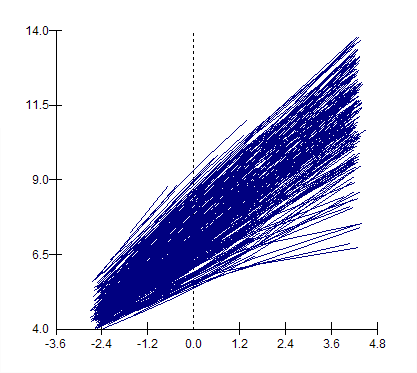
-2*log(lh) is 3132.02There’s very little variation left at level 1 (occasions), as most has been absorbed by the more complex model at level 2 (students). Try using the variance function to verify that the model produces a variance that increases quadratically with age. You may also try to reproduce the following plot showing the predicted curves for all students. (The estimate includes the MLE of the fixed effects as well as BLUPs of the student-level residuals.)
This graph is easier to produce using the GUI, but for reference here are the commands use to compute the prediction:
note Computing residuals requires several commands:
rfun
note want residuals at level 2
rlev 2
note we don't need the covariances
rcov 0
note we do need three columns for storing them
rout c301 c302 c303
note go ahead compute them
resi
note now predict using the fixed and random effects
predict "one" c301 "age" c302 "agesq" c303 c21
name c21 "prediction"
erase c301 c302 c303