
We now consider 3-level models. We will use time-series data on 1721 students nested within 60 urban public primary schools. The outcome of interest is mathematics achievement. The data were collected at the end of first grade and annually thereafter up to sixth grade, but not all students have six observations.
This dataset is used in Chapter 4 of the manual for HLM 6. It came in three files, one for each level, but I have merged them into a single file available in the course website.
A correspondent asked about the equations for the models fitted here. I have included links to the equations for the growth curve model, and for the growth curve model with predictors, skipping the simpler variance-components model.
We read the data and fit a simple variance-components model. Note that we have two specifications for the random part, one at the school level (level 3), and one at the child-level (level 2). They are both null (intercept-only) models, so we are simply adding an error term at each level. We specify these going down the hierarchy. We also specify maximum likelihood estimation. (The R default is REML).
. use https://grodri.github.io/datasets/egm, clear
(Data from HLM 6 manual on math achievement in 60 urban schools)

. mixed math || schoolid: || childid:  , mle

Performing EM optimization ...

Performing gradient-based optimization:
Iteration 0:   log likelihood = -12652.991
Iteration 1:   log likelihood =  -12652.99

Computing standard errors ...

Mixed-effects ML regression                     Number of obs     =      7,230

        Grouping information
        ────────────────┬────────────────────────────────────────────
                        │     No. of       Observations per group
         Group variable │     groups    Minimum    Average    Maximum
        ────────────────┼────────────────────────────────────────────
               schoolid │         60         18      120.5        387
                childid │      1,721          2        4.2          6
        ────────────────┴────────────────────────────────────────────

                                                Wald chi2(0)      =          .
Log likelihood =  -12652.99                     Prob > chi2       =          .

─────────────┬────────────────────────────────────────────────────────────────
        math │ Coefficient  Std. err.      z    P>|z|     [95% conf. interval]
─────────────┼────────────────────────────────────────────────────────────────
       _cons │   -.510021   .0779639    -6.54   0.000    -.6628275   -.3572144
─────────────┴────────────────────────────────────────────────────────────────

─────────────────────────────┬────────────────────────────────────────────────
  Random-effects parameters  │   Estimate   Std. err.     [95% conf. interval]
─────────────────────────────┼────────────────────────────────────────────────
schoolid: Identity           │
                  var(_cons) │    .317646   .0687236       .207866    .4854037
─────────────────────────────┼────────────────────────────────────────────────
childid: Identity            │
                  var(_cons) │   .5704854   .0337543      .5080202    .6406312
─────────────────────────────┼────────────────────────────────────────────────
               var(Residual) │   1.523894   .0290756      1.467959     1.58196
─────────────────────────────┴────────────────────────────────────────────────
LR test vs. linear model: chi2(2) = 1404.55               Prob > chi2 = 0.0000

Note: LR test is conservative and provided only for reference.
> library(haven)
> library(lme4)
> egm <- read_dta("https://grodri.github.io/datasets/egm.dta")
> vc <- lmer(math ~ 1 + (1|childid) + (1 | schoolid), data=egm, REML=FALSE)
> summary(vc, corr = FALSE)
Linear mixed model fit by maximum likelihood  ['lmerMod']
Formula: math ~ 1 + (1 | childid) + (1 | schoolid)
   Data: egm

     AIC      BIC   logLik deviance df.resid
 25314.0  25341.5 -12653.0  25306.0     7226

Scaled residuals:
    Min      1Q  Median      3Q     Max
-2.6726 -0.6576  0.0265  0.6735  3.3344

Random effects:
 Groups   Name        Variance Std.Dev.
 childid  (Intercept) 0.5705   0.7553
 schoolid (Intercept) 0.3176   0.5636
 Residual             1.5239   1.2345
Number of obs: 7230, groups:  childid, 1721; schoolid, 60

Fixed effects:
            Estimate Std. Error t value
(Intercept) -0.51002    0.07796  -6.542
We have 60 schools with an average of 120.5 students for a total of 1721 children, who have between 2 and 6 observations each for a total of 7230 observations.
Our estimate of the mean score is -0.51 and the standard deviations are 0.56, 0.76 and 1.23 at the school, child and observation levels. We can turns these into intraclass correlations from first principles.
. mat list e(b) // to get names

e(b)[1,4]
          math:   lns1_1_1:   lns2_1_1:    lnsig_e:
         _cons       _cons       _cons       _cons
y1  -.51002095  -.57340893  -.28063386   .21063435

. scalar v3 = exp(2 * _b[lns1_1_1:_cons])

. scalar v2 = exp(2 * _b[lns2_1_1:_cons])

. scalar v1 = exp(2 * _b[lnsig_e:_cons])

. display v3/(v3 + v2 + v1), (v2 + v3)/(v3 + v2 + v1)
.13169264 .36820984
> v <- c(sigma(vc)^2, unlist(VarCorr(vc)))
> v[3]/(v[1] + v[2] + v[3])
 schoolid
0.1316919
> (v[2] + v[3])/(v[1] + v[2] + v[3])
  childid
0.3682094
We find intra-class correlations of 0.13 at the school level and 0.37 at the child level. These numbers represent the correlation in math achievement between two children in the same school, and between two measurements on the same child (in the same school). We can also conclude that 13% of the variation in math achievement can be attributed to the schools and 37% to the children (which includes the school).
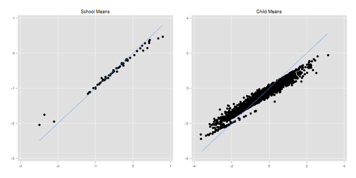
We can also obtain posterior Bayes estimates of the school and child random effects (these come up in the same order as the equations) and compare with school and child means
. predict r3 r2, reffects

. // 3
. egen m3 = mean(math), by(schoolid)

. gen eb3 = _b[_cons] + r3

. egen lev3 = tag(schoolid)

. twoway (scatter eb3 m3 if lev3) (function y=x, range(-2.5 .8)), ///
>   legend(off) title(School Means) name(school, replace)

. // 2
. egen m2 = mean(math), by (childid)

. egen n2 = count(math), by(childid) //?

. gen eb2 = eb3 + r2

. egen lev2 = tag(childid)

. twoway (scatter eb2 m2 if lev2 & n2 > 2) (function y=x, range(-3.6 3.1)), ///
>   legend(off) title(Child Means) name(child, replace)

. // graph
. graph combine school child, xsize(6) ysize(3)

. graph export egmfig1.png, width(700) replace
file egmfig1.png saved as PNG format
> library(dplyr)
> library(ggplot2)
> library(gridExtra)
> re <- ranef(vc)
> # schools
> schools  <- group_by(egm, schoolid) |>
+   summarize(ml3 = mean(math)) |>
+   mutate(eb3 = fixef(vc) + re$schoolid[schoolid, ] )
> r <- data.frame(x=range(schools$ml3))
> g3 <- ggplot(schools, aes(ml3, eb3)) + geom_point() +
+   geom_line(data=r, aes(x,x))
> # students
> students <- group_by(egm, childid) |>
+   summarize(ml2 = mean(math), schoolid = first(schoolid) ) |>
+   mutate(eb2 = fixef(vc) + re$schoolid[schoolid,1] + re$childid[childid,1])
> r <- data.frame(x=range(students$ml2))
> g2 <- ggplot(students, aes(ml2, eb2)) + geom_point() +
+   geom_line(data=r, aes(x,x))
> g <- arrangeGrob(g3, g2, ncol=2)
> ggsave("egmfig1r.png", plot = g, width=10, height=5, dpi=72)
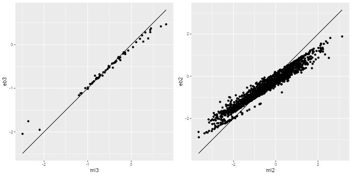
We see the usual shrinkage, particularly for the child means.
The obvious predictor at the observation level is study
year, which is coded -2.5, -1.5, -0.5, 0.5, 1.5 and 2.5 for
the six years of data collection. There’s also a variable called
grade reflecting the grade minus one, which is almost the
same thing:
. tab year grade

           │                         grade
      year │         0          1          2          3          4 │     Total
───────────┼───────────────────────────────────────────────────────┼──────────
      -2.5 │       131          0          0          0          0 │       131
      -1.5 │     1,346          0          0          0          0 │     1,346
       -.5 │       104      1,412          4          0          0 │     1,520
        .5 │         1        194      1,470          7          0 │     1,672
       1.5 │         0          5        174      1,200          8 │     1,387
       2.5 │         0          1          5        149      1,010 │     1,174
───────────┼───────────────────────────────────────────────────────┼──────────
     Total │     1,582      1,612      1,653      1,356      1,018 │     7,230


           │   grade
      year │         5 │     Total
───────────┼───────────┼──────────
      -2.5 │         0 │       131
      -1.5 │         0 │     1,346
       -.5 │         0 │     1,520
        .5 │         0 │     1,672
       1.5 │         0 │     1,387
       2.5 │         9 │     1,174
───────────┼───────────┼──────────
     Total │         9 │     7,230
> table(egm$year, egm$grade)

          0    1    2    3    4    5
  -2.5  131    0    0    0    0    0
  -1.5 1346    0    0    0    0    0
  -0.5  104 1412    4    0    0    0
  0.5     1  194 1470    7    0    0
  1.5     0    5  174 1200    8    0
  2.5     0    1    5  149 1010    9
We will follow the HLM manual in using years to track progress in math achievement over time. Year zero is near the start of the third grade, and I will refer to it as ‘third grade’ for simplicity.
Our first model will allow for random intercepts and slopes, with no
predictors at levels 2 or 3. I specify
covariance(unstructured) at each level, so the intercept
and slope can be correlated at level 2 as well as level 3.
The equations for this model are here.
. mixed math year ///
>   || schoolid: year, covariance(unstructured) ///
>   || childid:  year, covariance(unstructured) mle

Performing EM optimization ...

Performing gradient-based optimization:
Iteration 0:   log likelihood = -8169.1304
Iteration 1:   log likelihood = -8163.1176
Iteration 2:   log likelihood = -8163.1156
Iteration 3:   log likelihood = -8163.1156

Computing standard errors ...

Mixed-effects ML regression                     Number of obs     =      7,230

        Grouping information
        ────────────────┬────────────────────────────────────────────
                        │     No. of       Observations per group
         Group variable │     groups    Minimum    Average    Maximum
        ────────────────┼────────────────────────────────────────────
               schoolid │         60         18      120.5        387
                childid │      1,721          2        4.2          6
        ────────────────┴────────────────────────────────────────────

                                                Wald chi2(1)      =    2499.87
Log likelihood = -8163.1156                     Prob > chi2       =     0.0000

─────────────┬────────────────────────────────────────────────────────────────
        math │ Coefficient  Std. err.      z    P>|z|     [95% conf. interval]
─────────────┼────────────────────────────────────────────────────────────────
        year │   .7630273   .0152609    50.00   0.000     .7331164    .7929382
       _cons │  -.7793053   .0578295   -13.48   0.000    -.8926489   -.6659616
─────────────┴────────────────────────────────────────────────────────────────

─────────────────────────────┬────────────────────────────────────────────────
  Random-effects parameters  │   Estimate   Std. err.     [95% conf. interval]
─────────────────────────────┼────────────────────────────────────────────────
schoolid: Unstructured       │
                   var(year) │   .0110171   .0025621      .0069842    .0173788
                  var(_cons) │   .1653165   .0359122      .1079959    .2530611
             cov(year,_cons) │   .0170462   .0071472       .003038    .0310545
─────────────────────────────┼────────────────────────────────────────────────
childid: Unstructured        │
                   var(year) │   .0112561    .001961      .0080001    .0158373
                  var(_cons) │   .6404597    .025183      .5929559    .6917691
             cov(year,_cons) │   .0467854    .005063      .0368621    .0567086
─────────────────────────────┼────────────────────────────────────────────────
               var(Residual) │   .3014383   .0066403      .2887005    .3147382
─────────────────────────────┴────────────────────────────────────────────────
LR test vs. linear model: chi2(6) = 5595.58               Prob > chi2 = 0.0000

Note: LR test is conservative and provided only for reference.

. estat recov, corr

Random-effects correlation matrix for level schoolid

             │      year      _cons
─────────────+──────────────────────
        year │         1
       _cons │  .3994262          1

Random-effects correlation matrix for level childid

             │      year      _cons
─────────────+──────────────────────
        year │         1
       _cons │  .5510233          1
> gc <- lmer(math ~ year + (1 + year|childid) + (1 + year|schoolid),
+   data = egm, REML=FALSE)
> summary(gc)
Linear mixed model fit by maximum likelihood  ['lmerMod']
Formula: math ~ year + (1 + year | childid) + (1 + year | schoolid)
   Data: egm

     AIC      BIC   logLik deviance df.resid
 16344.2  16406.2  -8163.1  16326.2     7221

Scaled residuals:
    Min      1Q  Median      3Q     Max
-3.2047 -0.5640 -0.0372  0.5309  5.2629

Random effects:
 Groups   Name        Variance Std.Dev. Corr
 childid  (Intercept) 0.64046  0.8003
          year        0.01126  0.1061   0.55
 schoolid (Intercept) 0.16532  0.4066
          year        0.01102  0.1050   0.40
 Residual             0.30144  0.5490
Number of obs: 7230, groups:  childid, 1721; schoolid, 60

Fixed effects:
            Estimate Std. Error t value
(Intercept) -0.77930    0.05783  -13.48
year         0.76303    0.01526   50.00

Correlation of Fixed Effects:
     (Intr)
year 0.357
The first thing you will notice is that as models become more complex they take a bit longer to run. The results can be compared with the output from HLM 6 starting on page 80 of the manual, and are in very close agreement.
The fixed-effect estimates yield an intercept of -0.78 and a slope of 0.76. These values can be interpreted as the average achievement in third grade, and the average rate of change per year. Clearly average math achievement increases significantly over time.
The output also shows the variances and covariances of the random
effects. The correlations can be obtained with
estat recovariance, which has an option
corr.
We see that the intercepts and slopes have correlations of 0.40 at the school level and 0.55 at the child level. (In a hierarchical model the correlation at level 2 is never lower than at level 3.) The child estimate (0.55) can be interpreted as the correlation between a child’s achievement around third grade and her rate of growth. The school estimate (0.40) represents the correlation between a school’s achievement around third grade and the rate of change per year.
Most of the variance in the intercept comes from the child level, whereas the variance in the slope is about the same at each level. These results indicate fairly significant variation among schools in mean achievement around third grade, as well as in the rates of change over time.
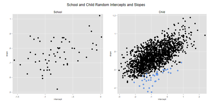
We can now estimate growth curves for each school and for each child,
combining the estimated fixed and random effects. I’ll just predict the
random effects, and plot the slope versus the intercept at each level.
Note that at the child level I include both the school and child
residuals. In Stata we use predict with
the reffects option. With four random effects we need four
variables to store the Bayes estimates. I’ll use numbers for the levels,
a for intercepts and b for slopes.
. predict r3b r3a r2b r2a, reffects

. local labels xtitle(intercept) ytitle(slope)

. gen a3 = _b[_cons] + r3a

. gen b3 = _b[year]  + r3b

. twoway scatter b3 a3 if lev3, `labels' title(School) ///
>   name(school, replace)

. gen a2 = a3 + r2a // or _b[_cons] + r3a + r2a

. gen b2 = b3 + r2b // or _b[year]  + r3b + r3b

. twoway (scatter b2 a2 if lev2, `labels') ///
>   (scatter b2 a2 if lev2 & b3 < .55), legend(off) ///
>   title(Child) name(child, replace)

. graph combine school child, xsize(6) ysize(3) ///
>   title(School and Child Random Intercepts and Slopes)

. graph export egmfig2.png, width(700) replace
file egmfig2.png saved as PNG format
> b = fixef(gc)
> gcre <- ranef(gc)
> names(gcre$schoolid) <- names(gcre$childid) <- c("intercept","slope")
> school <- mutate(gcre$schoolid, intercept = b[1] + intercept, slope = b[2] + slope)
> g3 <- ggplot(school, aes(intercept,slope)) + geom_point()
> child <- select(egm, schoolid, childid) |>
+   group_by(childid) |> filter(row_number()==1) |> mutate(
+   intercept = b[1] + gcre$schoolid[schoolid,1] + gcre$childid[childid,1],
+   slope     = b[2] + gcre$schoolid[schoolid,2] + gcre$childid[childid,2])
> g2 <- ggplot(child, aes(intercept,slope)) + geom_point() +
+   geom_point(data=filter(child, slope < .55), aes(intercept,slope), color="blue")
> g <- arrangeGrob(g3, g2, ncol=2)
> ggsave("egmfig2r.png", plot = g, width=10, height=5, dpi=72)
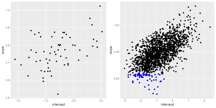
We see substantial variation in school levels and rates of change in math achievement. One school is notable for having a reasonable third-grade mean, but a low rate of change per year (just above 0.5). I highlight the children from this school in the graph on the right, which shows their expected third-grade scores and rates of change combining school and child effects.
Note the positive correlation between intercepts and slopes at both levels, so children and schools with higher third-grade math achievement also tend to show greater gains over time.
We can also plot fitted lines at the school and child level. It might not be a bad idea to test for linearity of the growth curves.
One way to look for school or individual characteristics that may be associated with levels and trends in mathematics achievement is to plot or regress the Bayes estimates of intercepts and slopes on potential predictors at each level.
Here I’ll follow the HLM manual in considering a model where a child’s growth curve depends on ethnicity, with different intercepts and slopes for whites, blacks and hispanics, and where the school average curve depends on the percent of students with low income.
One way to develop a model of this type is to write down the equation
for each level and then substitute down the hierarchy to obtain the
fixed and random components in the complete model. This process shows
the need to create cross-level interactions between year
and the predictors at the school and child level.
Before creating cross-products we consider centering. This is not needed (not, in my view, advisable) for dummy variables, where zero is meaningful because it identifies the reference category. One might consider centering the percent poor, but for consistency with the HLM manual I will not. Bear in mind that the main effects then refer to
The equations for this model are here.
. gen yearBlack = year * black

. gen yearHispanic = year * hispanic

. gen yearLowinc = year * lowinc

. mixed math year black hispanic lowinc ///
>   yearBlack yearHispanic yearLowinc ///
>   || schoolid: year, covariance(unstructured) ///
>   || childid:  year, covariance(unstructured) mle

Performing EM optimization ...

Performing gradient-based optimization:
Iteration 0:   log likelihood = -8125.8349
Iteration 1:   log likelihood = -8119.6062
Iteration 2:   log likelihood = -8119.6035
Iteration 3:   log likelihood = -8119.6035

Computing standard errors ...

Mixed-effects ML regression                     Number of obs     =      7,230

        Grouping information
        ────────────────┬────────────────────────────────────────────
                        │     No. of       Observations per group
         Group variable │     groups    Minimum    Average    Maximum
        ────────────────┼────────────────────────────────────────────
               schoolid │         60         18      120.5        387
                childid │      1,721          2        4.2          6
        ────────────────┴────────────────────────────────────────────

                                                Wald chi2(7)      =    3324.78
Log likelihood = -8119.6035                     Prob > chi2       =     0.0000

─────────────┬────────────────────────────────────────────────────────────────
        math │ Coefficient  Std. err.      z    P>|z|     [95% conf. interval]
─────────────┼────────────────────────────────────────────────────────────────
        year │   .8745122   .0391404    22.34   0.000     .7977984    .9512259
       black │  -.5021085   .0778753    -6.45   0.000    -.6547414   -.3494756
    hispanic │  -.3193816   .0860935    -3.71   0.000    -.4881218   -.1506414
      lowinc │  -.0075778   .0016908    -4.48   0.000    -.0108918   -.0042638
   yearBlack │  -.0309253   .0224586    -1.38   0.169    -.0749432    .0130927
yearHispanic │   .0430865    .024659     1.75   0.081    -.0052442    .0914172
  yearLowinc │  -.0013689   .0005226    -2.62   0.009    -.0023933   -.0003446
       _cons │   .1406379   .1274908     1.10   0.270    -.1092396    .3905153
─────────────┴────────────────────────────────────────────────────────────────

─────────────────────────────┬────────────────────────────────────────────────
  Random-effects parameters  │   Estimate   Std. err.     [95% conf. interval]
─────────────────────────────┼────────────────────────────────────────────────
schoolid: Unstructured       │
                   var(year) │   .0079801   .0020562       .004816    .0132231
                  var(_cons) │   .0780901    .019642      .0476973    .1278494
             cov(year,_cons) │   .0008172   .0044663     -.0079366     .009571
─────────────────────────────┼────────────────────────────────────────────────
childid: Unstructured        │
                   var(year) │   .0110938   .0019517      .0078583    .0156615
                  var(_cons) │   .6222512   .0245399      .5759658    .6722562
             cov(year,_cons) │   .0466258   .0049886      .0368483    .0564033
─────────────────────────────┼────────────────────────────────────────────────
               var(Residual) │   .3015912   .0066415      .2888511    .3148932
─────────────────────────────┴────────────────────────────────────────────────
LR test vs. linear model: chi2(6) = 4797.28               Prob > chi2 = 0.0000

Note: LR test is conservative and provided only for reference.
> egm <- mutate(egm, eth = factor(1 + black + 2 * hispanic,
+   labels=c("white","black","hispanic")))
> gcp <- lmer(math ~ year * (eth + lowinc) +
+   (year | childid) + (year | schoolid),  data=egm, REML=FALSE)
> summary(gcp, corr=FALSE)
Linear mixed model fit by maximum likelihood  ['lmerMod']
Formula: math ~ year * (eth + lowinc) + (year | childid) + (year | schoolid)
   Data: egm

     AIC      BIC   logLik deviance df.resid
 16269.2  16372.5  -8119.6  16239.2     7215

Scaled residuals:
    Min      1Q  Median      3Q     Max
-3.2482 -0.5645 -0.0328  0.5348  5.2766

Random effects:
 Groups   Name        Variance Std.Dev. Corr
 childid  (Intercept) 0.622249 0.78883
          year        0.011091 0.10531  0.56
 schoolid (Intercept) 0.078134 0.27952
          year        0.007979 0.08933  0.03
 Residual             0.301594 0.54918
Number of obs: 7230, groups:  childid, 1721; schoolid, 60

Fixed effects:
                   Estimate Std. Error t value
(Intercept)       0.1406281  0.1275156   1.103
year              0.8745121  0.0391388  22.344
ethblack         -0.5021177  0.0778780  -6.447
ethhispanic      -0.3193836  0.0860948  -3.710
lowinc           -0.0075776  0.0016911  -4.481
year:ethblack    -0.0309297  0.0224580  -1.377
year:ethhispanic  0.0430851  0.0246583   1.747
year:lowinc      -0.0013689  0.0005226  -2.619
optimizer (nloptwrap) convergence code: 0 (OK)
Model failed to converge with max|grad| = 0.00341218 (tol = 0.002, component 1)
Results can be compared with the HLM output starting on page 88 of the manual. In this model each child has her own growth curve, but the intercept and slope depend on the school’s percent poor, school unobserved characteristics, the child’s owh ethnicity, and unobserved characteristics of the child.
One way to think about the estimates is as follows. We start with a growth curve that has 0.141 points of math achievement by the middle of third grade and increases by 0.875 points per year, provided the school has no poor students. Each percentage point of low income students is associated with a third grade mean that’s 0.008 lower and increases 0.001 points less per year, so a school with 100% poor students would have a third-grade mean of -0.617 and an increase of 0.738 points per year. The intercept and slope in any particular school will vary around the average line for its percent poor.
Next come characteristics of the individual, in this case ethnicity. Blacks have a third-grade mean 0.502 points below whites in the same school, and the increase per year is 0.031 points less than for whites in the same school. The results for hispanics indicate a third-grade mean 0.319 points below whites, but a growth rate per year 0.043 points higher than whites in the same school. Each child’s growth curve, however, will vary around the average line for kids of the same ethnicity in the same school.
The random effects indicate that the average third-grade score varies by school, with a standard deviation of 0.28, while the rate of change has a standard deviation of 0.089. Interestingly, the correlation between intercept and slope has practically vanished, suggesting that it can be attributed to the school’s socio-economic composition.
Variation at the child level is even more sustantial; expected third-grade scores vary with a standard deviation of 0.789, and the rates of change vary with a standard deviation of 0.105. These two random effects remain highly correlated, so kids who have high levels of math proficiency in third grade also tend to improve faster over time.
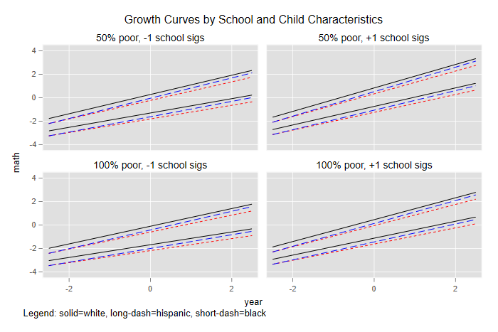
It’s useful to compare fixed and random effects on a similar scale. Here I will consider four types of schools, with 50 and 100 poor and random effects one standard deviation above and below the mean. In each school I will consider kids from the three ethnic groups whose intercepts and slopes fall one standard deviation above and below the mean of their ethnic group in their school.
To do this we need to create a prediction dataset with the combinations of interest. I will store these in the first few rows of the dataset.
. local k = 1

. foreach lowinc in 50 100 {
  2.   foreach eth in "white" "black" "hispanic" {
  3.     foreach year in -2.5 2.5 {
  4.       quietly replace lowinc   = `lowinc' in `k'
  5.       quietly replace black    = "`eth'" == "black" in `k'
  6.       quietly replace hispanic = "`eth'" == "hispanic" in `k'
  7.       quietly replace year     = `year' in `k'
  8.       local k = `k' + 1
  9.     }
 10.   }
 11. }

. keep in 1/12
(7,218 observations deleted)

. quietly replace yearBlack    = year * black

. quietly replace yearHispanic = year * hispanic

. quietly replace yearLowinc   = year * lowinc
> pdf <- data.frame(
+   lowinc   = rep(c(50,100),c(24,24)),
+   schoolz  = rep(rep(c(-1,1), c(12,12)),2),
+   black    = rep(rep(c(0,1,0),c(2,2,2)),8),
+   hispanic = rep(rep(c(0,0,1),c(2,2,2)),8),
+   childz   = rep(rep(c(-1,1),c(6,6)), 4),
+   year     = rep(c(-2.5,2.5), 24)
+ ) |> mutate(
+   eth = factor(1 + black + 2 * hispanic, labels=c("white","black","hispanic"))
+ )
We can then predict the fixed effects and add the random effects. In Stata we expand the dataset to add the random effects.
. predict xb, xb

. expand 4
(36 observations created)

. bysort lowinc  black hispanic year: gen rep=_n

. gen schoolz = -1 + 2 * (rep > 2)

. gen childz  = -1 + 2 * (rep == 2 | rep ==4)

. scalar sa3 = exp(_b[lns1_1_2:_cons]) // school cons

. scalar sa2 = exp(_b[lns2_1_2:_cons]) // child cons

. scalar sb3 = exp(_b[lns1_1_1:_cons]) // school year

. scalar sb2 = exp(_b[lns2_1_1:_cons]) // child year

. gen fv = xb + (schoolz * sa3 + childz * sa2) + ///
>   (schoolz * sb3 + childz * sb2) * year
> sdre <- rbind(attr(VarCorr(gcp)$schoolid,"stddev"),
+   attr(VarCorr(gcp)$childid,"stddev"))
> xb <- predict(gcp, newdata = pdf, re.form = ~0)
> pdf <- mutate(pdf,
+   xb = xb,
+   fv = xb +
+   (schoolz * sdre[1,1] + childz * sdre[2,1]) +
+   (schoolz * sdre[1,2] + childz * sdre[2,2]) * year
+ )
We are now ready to plot the results
. label define schoolz -1 "-1 school sigs" 1 "+1 school sigs"

. label values schoolz schoolz

. label define lowinc 50 "50% poor" 100 "100% poor"

. label values lowinc lowinc

. gen eth = 1 + black + 2*hispanic

. sort schoolz lowinc childz eth year

. twoway line fv year if eth == 1, c(asc) lpat(solid) ///
>   ||  line fv year if eth == 2, c(asc) lpat(shortdash) lc(red) ///
>   ||  line fv year if eth == 3, c(asc) lpat(dash) lc(blue) ///
> , by(lowinc schoolz, legend(off) ///
>   note("Legend: solid=white, long-dash=hispanic, short-dash=black") ///
>   title("Growth Curves by School and Child Characteristics")) ///
>   xtitle(year) ytitle(math)

. graph export egmfig3.png, width(700) replace
file egmfig3.png saved as PNG format
> ggplot(filter(pdf,childz==-1), aes(year, fv, linetype=eth)) +
+   geom_line() +
+   geom_line(data=filter(pdf,childz==1), aes(year, fv, linetype=eth)) +
+   facet_grid(lowinc ~ schoolz)
>   ggsave("egmfig3r.png", width=10, height=8, dpi=72)
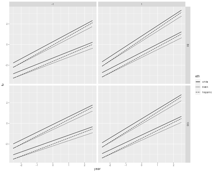
The plot shows the relative importance of fixed and random effects at the school and individual levels. At the school level the difference between 50% and 100% poor is smaller than the two-sigma difference in unobserved school characteristics. At the individual level the differences between whites, blacks and hispanics are dwarfed by the two-sigma differences in unobserved child characteristics. Interestingly, within each school type the average line for hispanics starts at about the average level of blacks in first grade, but catches up with the average level of whites by sixth grade.