Gibbs Sampling Using JAGS

JAGS is “Just Another Gibbs Sampler”, a program for the analysis of Bayesian models using MCMC. It uses essentially the same model language as WinBUGS or OpenBUGS. It works closely with R via rjags, so that’s what I will use here. Let’s try it.

We start by writing our model and saving it to a file, here hosp.bugs. This is exactly the same code used for WinBUGS here.

    model {
        # N observations
        for (i in 1:N) {
            hospital[i] ~ dbern(p[i])
            logit(p[i]) <- bcons + bloginc*loginc[i] + bdistance*distance[i] + 
                bdropout*dropout[i] + bcollege*college[i] + u[group[i]] 
        }
        # M groups
        for (j in 1:M) {
            u[j] ~ dnorm(0,tau)
        }
        # Priors
        bcons     ~ dnorm(0.0,1.0E-6)
        bloginc   ~ dnorm(0.0,1.0E-6)
        bdistance ~ dnorm(0.0,1.0E-6)
        bdropout  ~ dnorm(0.0,1.0E-6)
        bcollege  ~ dnorm(0.0,1.0E-6)
        # Hyperprior
        tau ~ dgamma(0.001,0.001)
    }

Next we need the data, which need to be in a list. We will read them into R just like we did here, and then produce a list with the number of observations (N) and groups (M), the outcome hospital and the predictors loginc, distance, dropout and college. We also need mother, which groups the births.

> hosp <- read.table("https://data.princeton.edu/pop510/hospital.dat", 
+     header = FALSE)
> names(hosp) <- c("hosp","loginc","distance","dropout","college","mother")
> hosp_data <- list(N = 1060, M = 501, hospital = hosp$hosp, 
+     loginc=hosp$loginc, distance=hosp$distance, dropout=hosp$dropout, 
+     college=hosp$college, group=hosp$mother)

The other thing we need are initial values. We use two lists, one for each chain, with values scattered around the mle’s. The random effects are generated by JAGS.

> hosp_inits= list(
+   list(bcons=-2.5, bloginc=0.50, bdistance=-0.05, bdropout=-1.6, bcollege=0.7, tau=0.8),
+   list(bcons=-2.8, bloginc=0.40, bdistance=-0.08, bdropout=-1.4, bcollege=0.9, tau=1.2)
+ )

We are now ready. We load the rjags library and then compile the model by calling the jags.model() function

> library(rjags)
> model <- jags.model("hosp.bugs", data = hosp_data, inits =hosp_inits, n.chains=2)
Compiling model graph
   Resolving undeclared variables
   Allocating nodes
Graph information:
   Observed stochastic nodes: 1060
   Unobserved stochastic nodes: 507
   Total graph size: 9884

Initializing model

With the model ready we run a burn-in of 1000 iterations using update()

> update(model, n.iter = 1000)

We can now run a further 5000 iterations monitoring the parameters of interest. We use coda.samples(), which is a wrapper around jags.samples().

> samples <- coda.samples(model, 
+   variable.names = c("bcons","bloginc","bdistance","bdropout","bcollege","tau"), 
+   n.iter = 5000)

We can then summarize our samples, an object of class mcmc.list.

> summary(samples)

Iterations = 2001:7000
Thinning interval = 1 
Number of chains = 2 
Sample size per chain = 5000 

1. Empirical mean and standard deviation for each variable,
   plus standard error of the mean:

              Mean      SD  Naive SE Time-series SE
bcollege   1.05639 0.41282 0.0041282      0.0111317
bcons     -3.38305 0.50784 0.0050784      0.0508158
bdistance -0.07783 0.03281 0.0003281      0.0009328
bdropout  -2.04407 0.26939 0.0026939      0.0110984
bloginc    0.56473 0.07779 0.0007779      0.0072873
tau        0.63297 0.20605 0.0020605      0.0165996

2. Quantiles for each variable:

             2.5%      25%      50%      75%    97.5%
bcollege   0.2724  0.77612  1.04772  1.32113  1.89939
bcons     -4.4508 -3.70556 -3.35383 -3.02013 -2.49771
bdistance -0.1419 -0.09954 -0.07816 -0.05561 -0.01281
bdropout  -2.5991 -2.21880 -2.02912 -1.85405 -1.54798
bloginc    0.4204  0.51167  0.56040  0.61474  0.72825
tau        0.3291  0.48709  0.59592  0.74515  1.13837

The class also has a plot() method to produce the usual trace and density plots. R will pause between plots, but R Studio does not.

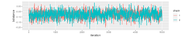
A good way to do a trace plot is to change the aspect ratio. I had good results with the following code

> library(dplyr)
> library(ggplot2)
> mcmc <- data.frame(rbind(samples[[1]], samples[[2]]))
> mcmc <- mutate(mcmc, 
+   chain=factor(rep(c(1,2),c(5000,5000))),
+   iteration = rep(1:5000, 2))
> r <- 5000 / (5*range(mcmc$bdistance) %*% c(-1,1) )
> ggplot(mcmc, aes(iteration, bdistance, color=chain)) + geom_line() + 
+   coord_fixed(ratio=r)
> ggsave("jagsFig1.png", width=500/72, height=400/72, dpi=72)

Which produces this plot:

References

Lunn D, Spiegelhalter D, Thomas A, Best N. (2009) The BUGS project: Evolution, critique and future directions. Statistics in Medicine, 28:3049-67.

Plummer M, Best N, Cowles K, Vines K (2006). CODA: Convergence Diagnosis and Output Analysis for MCMC, R News, 6:7-11. CRAN

Plummer, M, A. Stukalov, and M. Denwood (2022). Bayesian Graphical Models using MCMC. An R vignette. CRAN