
R can handle several types of data, including numbers, character strings, vectors and matrices, as well as more complex data structures. In this section I describe data frames, the preferred way to organize data for statistical analysis, explain how to read data from an external file into a data frame, and show how to examine the data using simple descriptive statistics and informative plots.
An important data structure that we have not discussed so far is the list. A list is a set of objects that are usually named and can be anything: numbers, character strings, matrices or even lists.
Unlike a vector, whose elements must all be of the same type (all
numeric, or all character), the elements of a list may have different
types. Here’s a list with two components created using the function
list():
> person <- list(name="Jane", age=24)Typing the name of the list prints all elements.
> person$name
[1] "Jane"
$age
[1] 24You can extract a component of a list using the extract operator
$. For example we can list just the name or
age of this person:
> person$name[1] "Jane"> person$age[1] 24Individual elements of a list can also be accessed using their
indices or their names as subscripts. For example we can get the name
using person[1] or person["name"]. You can use
single or double square brackets. If you use single brackets, as we did
here, you get a list with the name. If you use double brackets you get
just the name. Try person[[1]] or
person[["name"]] to see the difference.
A data frame is essentially a rectangular array containing the values of one or more variables for a set of units. The frame also contains the names of the variables, the names of the observations, and information about the nature of the variables, including whether they are numerical or categorical.
Internally, a data frame is a special kind of list, where each element is a vector of observations on a variable. Data frames look like matrices, but can have columns of different types. This makes them ideally suited for representing datasets, where some variables can be numeric and others can be categorical.
Data frames (like matrices) can also accommodate missing values,
which are coded using the special symbol NA. Most
statistical procedures, however, omit all missing values.
Data frames can be created from vectors, matrices or lists using the
function data.frame(), but more often than not one will
read data from an external file, as shown in the next two sections.
Free-format data are text files containing numbers or character strings separated by spaces. Optionally the file may have a header containing variable names. Here’s an excerpt of a data file containing information on three variables for 20 countries in Latin America:
              setting  effort   change
Bolivia            46       0        1
Brazil             74       0       10
Chile              89      16       29
  ... lines omitted ...
Venezuela          91       7       11
This small dataset includes an index of social setting, an index of
family planning effort, and the percent decline in the crude birth rate
between 1965 and 1975. The data are available on my website in a file
called effort.dat that includes a header with the variable
names.
R can read the data directly from the web:
> fpe <- read.table("https://grodri.github.io/datasets/effort.dat")The function used to read data frames is read.table().
The argument is a character string giving the name of the file
containing the data, but here we have given it a fully qualified url
(uniform resource locator), and that’s all it takes.
Alternatively, you could download the data and save them in a local
file, or just cut and paste the data from the browser to an editor, and
then save them. Make sure the file ends up in R’s working directory,
which you can find out by typing getwd(). If that is not
the case, you can use a fully qualified path name or change R’s working
directory by calling setwd() with a string argument.
Remember to double up your backward slashes (or use forward slashes
instead) when specifying paths in Windows.
Here we assigned the data to an object called fpe. To
print the object you simply type its name
> fpe setting effort change
Bolivia 46 0 1
Brazil 74 0 10
Chile 89 16 29
Colombia 77 16 25
CostaRica 84 21 29
Cuba 89 15 40
DominicanRep 68 14 21
Ecuador 70 6 0
ElSalvador 60 13 13
Guatemala 55 9 4
Haiti 35 3 0
Honduras 51 7 7
Jamaica 87 23 21
Mexico 83 4 9
Nicaragua 68 0 7
Panama 84 19 22
Paraguay 74 3 6
Peru 73 0 2
TrinidadTobago 84 15 29
Venezuela 91 7 11In this example R detected correctly that the first line in our file
was a header with the variable names. It also inferred correctly that
the first column had the observation names. (Well, it did so with a
little help; I made sure the row names did not have embedded spaces,
hence CostaRica. Alternatively, I could have used
"Costa Rica" in quotes as a row name.)
You can always tell R explicitly whether or not you have a header by
specifying the optional argument header=TRUE or
header=FALSE to the read.table() function.
This is important if you have a header but lack row names, because R’s
guess is based on the fact that the header line has one fewer entry than
the next row, as it did in our example.
If your file does not have a header line, R will use the default
variable names V1, V2, …, etc. To override
this default use read.table()’s optional argument
col.names to assign variable names. This argument takes a
vector of names. So, if our file did not have a header we could
have used the command
> fpe <- read.table("noheader.dat", col.names=c("setting","effort","change"))Don’t worry if this command doesn’t fit in a line. R code can be
continued automatically in a new line simply by making it obvious that
we are not done, for example ending the line with a comma, or having an
unclosed left parenthesis. R responds by prompting for more with the
continuation symbol + instead of the usual prompt
>.
If your file does not have observation names, R will simply number
the observations from 1 to n. You can specify row names using
read.table()’s optional argument row.names,
which works just like col.names; type
?data.frame for more information. (I should mention that in
a “tidy” world row names should just be another column, but classic R
treats them as observation indices.)
There are two closely related functions that can be used to get or
set variable and observation names at a later time. These are
called names(), for the variable or column names, and
row.names() for the observation or row names. Thus, if our
file did not have a header we could have read the data and then changed
the default variable names using the names() function:
> fpe <- read.table("noheader.dat")
> names(fpe) <- c("setting","effort","change")
Technical Note: If you have a background in other programming languages, you may be surprised to see a function call on the left hand side of an assignment. These are special replacement functions in R. They extract an element of an object and then replace its value.
In our example all three-variables were numeric. R will handle categorical variables with no problem, including factors and string variables. In Section 4 we will create a factor, basically a categorical variable that takes one of a finite set of values called levels, by grouping a numeric covariate into categories. In Section 5 we will read a dataset that includes string variables with values such as “low” and “high”. These can be converted to factors or kept as character data.
Exercise: Use a text editor to create a small file with the following three lines:
a b c
1 2 3
4 5 6
Read this file into R so the variable names are a,
b and c. Now delete the first row in the file,
save it, and read it again into R so the variable names are still
a, b and c.
Suppose the family planning effort data had been stored in a file containing only the actual data (no country names or variable names) in a fixed format, with social setting in character positions (often called columns) 1-2, family planning effort in positions 3-4 and fertility change in positions 5-6. This is a fairly common way to organize large datasets.
The following call will read the data into a data frame and name the variables:
> fpe <- read.table("fixedformat.dat",  col.names = c("setting", "effort",
"change"), sep=c(1, 3, 5))
Here I assume that the file in question is called
fixedformat.dat. I assign column names just as before,
using the col.names parameter. The novelty lies in the next
argument, called sep, which is used to indicate how the
variables are separated. The default is white space, which is
appropriate when the variables are separated by one or more blanks or
tabs. If the data are separated by commas, a common format with
spreadsheets, you can specify sep = ",". Here I created a
vector with the numbers 1, 3 and 5 to specify the character position (or
column) where each variable starts. Type ?read.table for
more details.
You can refer to any variable in the fpe data frame
using the extract operator $. For example to look at the
values of the fertility change variable, type
> fpe$change [1] 1 10 29 25 29 40 21 0 13 4 0 7 21 9 7 22 6 2 29 11and R will list a vector with the values of change for the 20
countries. You can also define fpe as your default dataset
by “attaching” it to your session:
> attach(fpe)If you now type the name effort by itself, R will now
look for it in the fpe data frame. If you are done with a
data frame, you can detach it using detach(fpe). While
attach() can save typing, experience has shown that it can
also lead to problems, suggesting it is best avoided. For example, if
you already have an object named effort, that will mask the
object in fpe. My advice is to always specify the data
frame name, as we do below.
To obtain simple descriptive statistics on these variables try the
summary() function:
> summary(fpe) setting effort change
Min. :35.0 Min. : 0.00 Min. : 0.00
1st Qu.:66.0 1st Qu.: 3.00 1st Qu.: 5.50
Median :74.0 Median : 8.00 Median :10.50
Mean :72.1 Mean : 9.55 Mean :14.30
3rd Qu.:84.0 3rd Qu.:15.25 3rd Qu.:22.75
Max. :91.0 Max. :23.00 Max. :40.00 As you can see, we get the min and max, 1st and 3rd quartiles, median
and mean. For categorical variables you get a table of counts.
Alternatively, you may ask for a summary of a specific variable. Or use
the functions mean() and var() for the mean
and variance of a variable, or cor() for the correlation
between two variables, as shown below:
> mean(fpe$effort)[1] 9.55> cor(fpe$effort, fpe$change)[1] 0.8008299Elements of data frames can be addressed using the subscript notation introduced in Section 2.3 for vectors and matrices. For example to list the countries that had a family planning effort score of zero we can use
> fpe[fpe$effort == 0, ] setting effort change
Bolivia 46 0 1
Brazil 74 0 10
Nicaragua 68 0 7
Peru 73 0 2This works because the expression fpe$effort == 0
selects the rows (countries) where the effort score is zero, while
leaving the column subscript blank selects all columns (variables).
The fact that the rows are named allows yet another way to select elements: by name. Here’s how to print the data for Chile:
> fpe["Chile", ] setting effort change
Chile 89 16 29Exercise: Can you list the countries where social setting is
high (say above 80) but effort is low (say below 10)? Hint: recall the
element-by-element logical operator &.
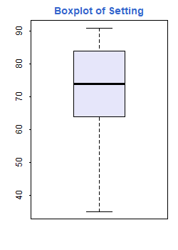
Probably the best way to examine the data is by using graphs. Here’s
a boxplot of setting. Inspired by a demo included in the R distribution,
I used custom colors for the box (“lavender”, specified using a name R
recognizes) and the title (#3366CC).
As noted earlier, R can save a plot as a png or jpeg file, so that it can be included directly on a web page. Other formats available are postscript for printing and windows metafile for embedding in other applications. Note also that you can cut and paste a graph to insert it in another document.
> boxplot(fpe$setting, col="lavender")
> title("Boxplot of Setting", col.main="#3366CC")
Here’s a scatterplot of change by effort, so you can see what a correlation of 0.80 looks like:
> plot(fpe$effort, fpe$change, pch=21, bg="gold")
> title("Scatterplot of Change by Effort", col.main="#3366CC")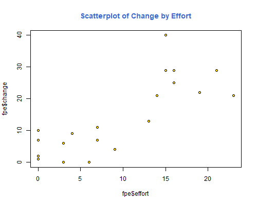
I used two optional arguments that work well together:
pch=21 selects a special plotting symbol, in this case a
circle, that can be colored and filled; and bf="gold"
selects the fill color for the symbol. I left the perimeter black, but
you can change this color with the col argument.
To identify points in a scatterplot use the identify()
function. Try the following on the graph window:
> identify(fpe$effort, fpe$change, row.names(fpe), ps = 9)The first three parameters to this function are the x and y
coordinates of the points and the character strings to be used in
labeling them. The ps optional argument specifies the size
of the text in points; here I picked 9-point labels.
Now click within a quarter of an inch of the points you want to
identify. R Studio will note that “locator is active”. When you are done
clicking press the Esc key. The labels will then appear
next to the points you clicked on. (If you are using the R GUI, the
labels will appear as you click on the points.)
Which country had the most effort but only moderate change? Which one had the most change?
Another interesting plot to try is pairs(), which draws
a scatterplot matrix. In our example try
pairs(fpe)
title("Scatterplots for Setting, Effort and Change", col.main="#3366CC")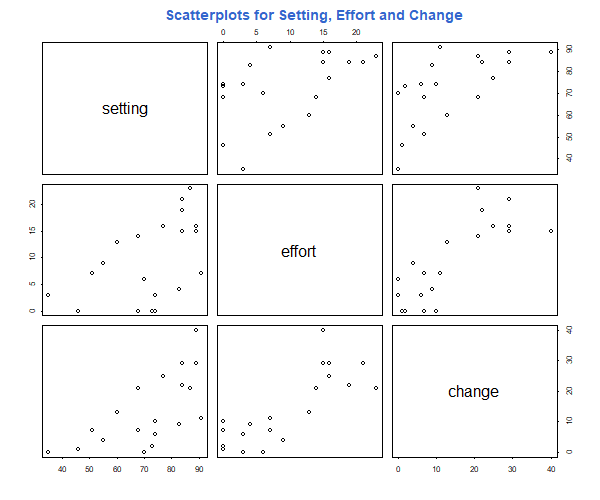
The result is a 3 by 3 matrix of scatterplots, with the variable names down the diagonal and plots of each variable against every other one.
Before you quit this session consider saving the fpe
data frame. To do this use the save() function
> save(fpe, file="fpe.Rdata")
> load("fpe.Rdata")
The first argument specifies the object to be saved, and the
file argument provides the name of a file, which will be in
the working directory unless a full path is given. (Remember to
double-up your backslashes in Windows, or use forward slashes
instead.)
By default R saves objects using a compact binary format which is
portable across all R platforms. There is an optional argument
ascii that can be set to TRUE to save the
object as ASCII text. This option was handy to transfer R objects across
platforms, but is no longer needed.
You can also save an image of your entire workspace, including all objects you have defined, and then load everything again, using
> save.image(file = "workspace.Rdata")
> load("workspace.Rdata")
In R Studio you can also do this using the Environment tab on the top
right; click on the floppy disk image to save the workspace, or on the
folder with an arrow to load a workspace. (In the R Gui you can use the
main menu; choose File|Save and
File|Load.)
When you quit R using q() you will be prompted to save
the workspace, unless you skip this safeguard by typing
q("no").
Exercise: Use R to create a scatterplot of change by setting, cut and paste the graph into a document in your favorite word processor, and try resizing and printing it. I recommend that you use the windows metafile format for the cut and paste operation.
Continue with Linear Models