
Let us try some linear models, starting with multiple regression and
analysis of covariance models, and then moving on to models using
regression splines. In this section I will use the data read in Section
3, so make sure the fpe data frame is still available (or
read it again).
To fit an ordinary linear model with fertility change as the response and setting and effort as predictors, try
> lmfit <- lm( change ~ setting + effort, data = fpe )Note first that lm() is a function, and we assign the
result to an object that I choose to call lmfit (for linear
model fit). This stores the results of the fit for later
examination.
The first argument to lm() is a model formula, which has
the response on the left of the tilde ~ (read “is modeled
as”), and a Wilkinson-Rogers model specification formula on the right. R
uses
+ to combine elementary terms, as in
A + B
: for interactions, as in A:B;
* for both main effects and interactions, so
A * B = A + B + A:B
A nice feature of R is that it lets you create interactions between categorical variables, between categorical and continuous variables, and even between numeric variables (it just creates the cross-product).
We also used the data argument to specify the data frame
containing these variables.
Let us look at the results of the fit. One thing you can do with
lmfit, as you can with any R object, is print it.
> lmfit
Call:
lm(formula = change ~ setting + effort, data = fpe)

Coefficients:
(Intercept)      setting       effort
   -14.4511       0.2706       0.9677
The output includes the model formula and the coefficients. You can
get a bit more detail by using the summary() function:
> summary(lmfit)
Call:
lm(formula = change ~ setting + effort, data = fpe)

Residuals:
     Min       1Q   Median       3Q      Max
-10.3475  -3.6426   0.6384   3.2250  15.8530

Coefficients:
            Estimate Std. Error t value Pr(>|t|)
(Intercept) -14.4511     7.0938  -2.037 0.057516 .
setting       0.2706     0.1079   2.507 0.022629 *
effort        0.9677     0.2250   4.301 0.000484 ***
---
Signif. codes:  0 '***' 0.001 '**' 0.01 '*' 0.05 '.' 0.1 ' ' 1

Residual standard error: 6.389 on 17 degrees of freedom
Multiple R-squared:  0.7381,    Adjusted R-squared:  0.7073
F-statistic: 23.96 on 2 and 17 DF,  p-value: 1.132e-05
The output includes a more conventional table with parameter
estimates and standard errors, as well the residual standard error and
multiple R-squared. (You could also get the matrix of correlations among
parameter estimates, by adding the option
correlation = TRUE in the call to summary(),
but that is a bit too much detail.)
To get a hierarchical analysis of variance table corresponding to
introducing each of the terms in the model one at a time, in the same
order as in the model formula, try the anova()
function:
> anova(lmfit)Analysis of Variance Table
Response: change
Df Sum Sq Mean Sq F value Pr(>F)
setting 1 1201.08 1201.08 29.421 4.557e-05 ***
effort 1 755.12 755.12 18.497 0.0004841 ***
Residuals 17 694.01 40.82
---
Signif. codes: 0 '***' 0.001 '**' 0.01 '*' 0.05 '.' 0.1 ' ' 1Alternatively, you can plot the results using
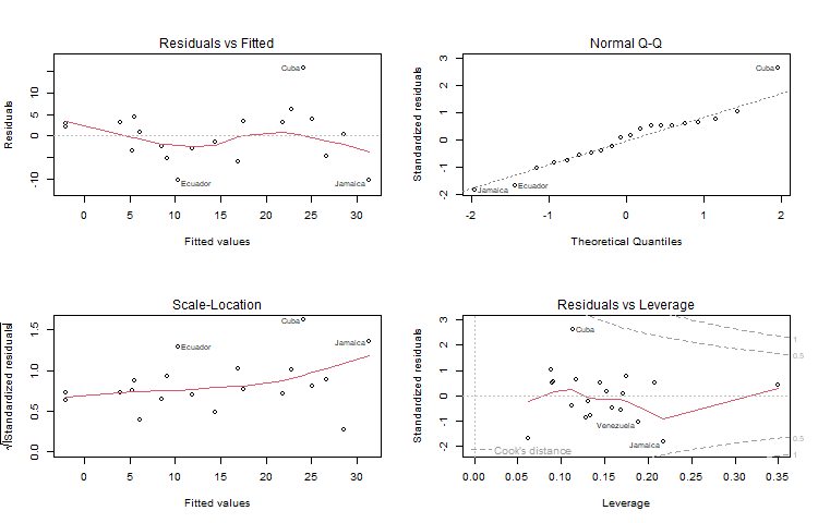
plot(lmfit)This will produce a set of four plots: residuals versus fitted values, a Q-Q plot of standardized residuals, a scale-location plot (square roots of standardized residuals versus fitted values, and a plot of residuals versus leverage, that adds bands corresponding to Cook’s distances of 0.5 and 1.
R Studio (and R) will prompt you to press Enter before showing each
graph, but we can do better. Type par(mfrow = c(2, 2)) to
set your graphics window to show four plots at once, in a layout with 2
rows and 2 columns. Then redo te graph using plot(lmfit).
To go back to a single graph per window use
par(mfrow = c(1, 1)). There are many other ways to
customize your graphs by setting high-level parameters, type
?par to learn more.
Technical Note: You may have noticed that we have used the
function plot() with all kinds of arguments: one or two
variables, a data frame, and now a linear model fit. In R jargon,
plot() is a generic function. It checks for the
kind of object that you are plotting, and then calls the appropriate
(more specialized) function to do the work. There are actually many plot
functions in R, including plot.data.frame() and
plot.lm(), and you can let R figure out which one to
call.
There are some specialized functions that allow you to extract elements from a linear model fit. For example
> fitted(lmfit) Bolivia Brazil Chile Colombia CostaRica
-2.004026 5.572452 25.114699 21.867637 28.600325
Cuba DominicanRep Ecuador ElSalvador Guatemala
24.146986 17.496913 10.296380 14.364491 9.140694
Haiti Honduras Jamaica Mexico Nicaragua
-2.077359 6.122912 31.347518 11.878604 3.948921
Panama Paraguay Peru TrinidadTobago Venezuela
26.664898 8.475593 5.301864 22.794043 16.946453 extracts the fitted values. In this case it will also print them,
because we did not asign them to anything. (The longer form
fitted.values() is an alias.)
To extract the coefficients use the coef() function (or
the longer form coefficients())
> coef(lmfit)(Intercept) setting effort
-14.4510978 0.2705885 0.9677137 To get the residuals, use the resids() function (or the
longer form residuals()). There is a type
argument that lets you choose several types of residuals, type
?residuals.lm for information. I find more useful the
rstudent() function that returns standardized
residuals:
> rstudent(lmfit) Bolivia Brazil Chile Colombia CostaRica
0.51666939 0.75316960 0.63588630 0.50233619 0.06666317
Cuba DominicanRep Ecuador ElSalvador Guatemala
3.32236668 0.56318276 -1.76471053 -0.22267614 -0.85483603
Haiti Honduras Jamaica Mexico Nicaragua
0.39308668 0.14477900 -1.98177567 -0.47988042 0.50479726
Panama Paraguay Peru TrinidadTobago Venezuela
-0.77508737 -0.40082283 -0.55507263 1.01832414 -1.03565220 If you are curious to see exactly what a linear model fit produces, try the function
> names(lmfit) [1] "coefficients" "residuals" "effects" "rank"
[5] "fitted.values" "assign" "qr" "df.residual"
[9] "xlevels" "call" "terms" "model" which lists the named components of a linear fit. All of these
objects may be extracted using the $ operator. However, if
there is a special extractor function such as coef() or
resid(), you are encouraged to use it.
So far our predictors have been continuous variables or covariates. We can also use categorical variables or factors. Let us group family planning effort into three categories:
> fpe$effortg <- cut(fpe$effort, breaks = c(-1, 4, 14, 100),
+   label = c("weak", "moderate", "strong"))
The function cut() creates a factor or categorical
variable. The first argument is an input vector, the second is a vector
of breakpoints, and the third is a vector of category labels. Note that
there is one more breakpoint than there are categories. All values
greater than the i-th breakpoint and less than or equal to the
(i+1)-st breakpoint go into the i-th category. Any
values below the first breakpoint or above the last one are coded
NA (a special R code for missing values). If the labels are
omitted, R generates a suitable default of the form “(a, b]”. By default
the intervals are closed on the right, so our intervals are \(\le 4\), 5-14, and 15+. To change this
behavior, use the option right = FALSE.
Note that by specifying fpe$effortg on the
left-hand-side, we have effectively added a new column to the
fpe data frame.
Try fitting the analysis of covariance model:
> covfit <- lm( change ~ setting + effortg, data = fpe)
> covfit
Call:
lm(formula = change ~ setting + effortg, data = fpe)

Coefficients:
    (Intercept)          setting  effortgmoderate    effortgstrong
        -5.9540           0.1693           4.1439          19.4476
As you can see, effortg has been treated automatically
as a factor, and R has generated the necessary dummy variables for
“moderate” and “strong” programs, treating “weak” as the reference
cell.
Choice of Contrasts: R codes unordered factors using the
reference cell or “treatment contrast” method. The reference cell is
always the first category which, depending on how the factor was
created, is usually the first in alphabetical order. If you don’t like
this choice, R provides a special function to re-order levels, check out
help(relevel).
You can obtain a hierarchical anova table for the analysis of
covariance model using the anova() function:
> anova(covfit)Analysis of Variance Table
Response: change
Df Sum Sq Mean Sq F value Pr(>F)
setting 1 1201.08 1201.08 36.556 1.698e-05 ***
effortg 2 923.43 461.71 14.053 0.0002999 ***
Residuals 16 525.69 32.86
---
Signif. codes: 0 '***' 0.001 '**' 0.01 '*' 0.05 '.' 0.1 ' ' 1Type ?anova to learn more about this function.
The real power of R begins to shine when you consider some of the
other functions you can include in a model formula. For starters, you
can include mathematical functions, for example
log(setting) is a perfectly legal term in a model formula.
You don’t have to create a variable representing the log of setting and
then use it, R will create it ‘on the fly’, so you can type
> lm( change ~ log(setting) + effort, data = fpe)
Call:
lm(formula = change ~ log(setting) + effort, data = fpe)

Coefficients:
 (Intercept)  log(setting)        effort
     -61.737        15.638         1.002
If you wanted to use orthogonal polynomials of degree 3 on setting,
you could include a term of the form poly(setting, 3).
You can also get R to calculate a well-conditioned basis for
regression splines. First you must load the splines
library.
> library(splines)This makes available the function bs() to generate
B-splines. For example the call
> fpe$setting.bs <- bs(fpe$setting, knots = c(66, 74, 84))will generate cubic B-splines with interior knots placed at 66, 74
and 84. This basis will use seven degrees of freedom, four corresponding
to the constant, linear, quadratic and cubic terms, plus one for each
interior knot. Alternatively, you may specify the number of degrees of
freedom you are willing to spend on the fit using the parameter
df. For cubic splines R will choose df-4 interior knots
placed at suitable quantiles. You can also control the degree of the
spline using the parameter degree, the default being
cubic.
If you like natural cubic splines, you can obtain a well-conditioned
basis using the function ns(), which has exactly the same
arguments as bs() except for degree, which is
always three. To generate a natural spline with five degrees of freedom,
use the call
> fpe$setting.ns <- ns(fpe$setting, df=5)Natural cubic splines are better behaved than ordinary splines at the extremes of the range. The restrictions mean that you save four degrees of freedom. You will probably want to use two of them to place additional knots at the extremes, but you can still save the other two.
To fit an additive model to fertility change using natural cubic splines on setting and effort with only one interior knot each, placed exactly at the median of each variable, try the following call:
> splinefit <- lm( change ~ ns(setting, knot=median(setting)) +
+   ns(effort, knot=median(effort)), data = fpe )
Here we used the parameter knot to specify where we
wanted the knot placed, and the function median() to
calculate the median of setting and effort. All calculations are done
“on the fly”.
Do you think the spline model is a good fit? Natural cubic splines with exactly one interior knot require the same number of parameters as an ordinary cubic polynomial, but are much better behaved at the extremes.
The lm() function has several additional parameters that
we have not discussed. These include
subset to restrict the analysis to a subset of the
dataweights to do weighted least squaresand many others; see help(lm) for further details. The
args() function lists the arguments used by any function,
in case you forget them. Try args(lm).
The fact that R has powerful matrix manipulation routines means that one can do many of these calculations from first principles. The next couple of lines create a model matrix to represent the constant, setting and effort, and then calculate the OLS estimate of the coefficients as \((X'X)^{-1}X'y:\)
> X <- cbind(1, fpe$effort, fpe$setting)
> solve( t(X) %*% X ) %*% t(X) %*% fpe$change
[,1]
[1,] -14.4510978
[2,] 0.9677137
[3,] 0.2705885Compare these results with coef(lmfit).
Continue with Generalized Linear Models