The Box-Cox Transformation

We will determine the optimal transformation for the analysis of covariance model of Section 2.8.

Venables and Ripley’s MASS library has a handy boxcox function, that computes and plots the profile log-likelihood for a range of possible transformations, going from -2 to 2. The main argument to the function is a linear model fit. We’ll try it with the analysis of covariance model of Section 2.8, that treats setting linearly and effort as a factor with three levels:

> library(MASS)

Warning: package 'MASS' was built under R version 4.2.2

Attaching package: 'MASS'

The following object is masked from 'package:dplyr':

    select

> bcm <-lm(y ~ setting + effort_g, data=fpe)
> png("fig28r.png", width=500, height=400)
> bc <- boxcox(bcm)
> dev.off()

png 
  2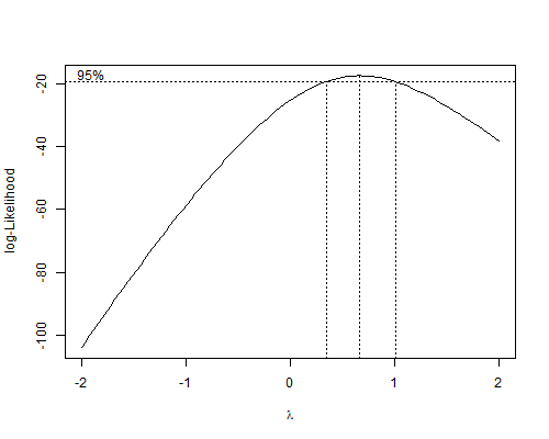 

As you can see from the graph, the optimal transformation has a parameter somewhat below 1, suggesting something like a square root transformation, but the profile log-likelihood is rather flat near the maximum, and leaving the data untransformed does not lower the log-likelihood significantly.

The boxcox function returns a list with x as the parameter and y as the corresponding log-likelihood. We can find the approximate mle as the x-value that yields the maximum:

> bc$x[bc$y == max(bc$y)]

[1] 0.6666667

So the optimal transformation is actually 0.67. In general I prefer to take this procedure has providing general guidance, and would pick something closer to reciprocals, logs, no transformation or squares, which correspond to values of -1, 0, 1 and 2, respectively. If one insisted on transforming the data, taking square roots would probably be best.

A large sample test for no transformation compares the log-likelihoods at one and at the maximum. Unfortunately 1 is not one of the generated x-values, but we can call the boxcox() function with a single parameter value to just evaluate the log-likelihood:

> bc1 <- boxcox(bcm, lambda=1, plotit=FALSE)
> -2*(bc1$y - max(bc$y))

[1] 3.645258

The chi-squared value 0f 3.65 is below the five-percent critical value, showing that we have no evidence against leaving the data in the original scale. To test for a log transformation you could use the same procedure, but it is clear from the graph that using logs would produce a substantially lower log-likelihood than leaving the data as they are.

Atkinson’s Score Test

Our final calculation involves Atkinson’s score test, which requires fitting the auxiliary variable given in Equation 2.31 in the notes. We compute the geometric mean, storing it in a scalar called gmean, use this to compute the auxiliary variable atkinson, and then fit the extended model:

> gmean <- exp(mean(log(fpe$y)))
> fpe <- mutate(fpe, atkinson = y * (log(y/gmean) - 1))
> lm(change ~ setting + effort_g + atkinson, data=fpe)

Call:
lm(formula = change ~ setting + effort_g + atkinson, data = fpe)

Coefficients:
     (Intercept)           setting  effort_gModerate    effort_gStrong          atkinson  
         -3.8582            0.1970            3.7850           11.6664            0.5916  

The coefficient of the auxiliary variable is 0.59, so the optimal power is approximately 1-0.59 = 0.41, suggesting again that something like a square root transformation might be indicated. The associated t-statistic is significant at the two percent level, but the more accurate likelihood ratio test statistic calculated earlier was not. Thus, we do not have strong evidence against keeping the response in the original scale.

Exercise 1: Try the Box-Tidwell procedure described in Section 2.10.4 of the notes to see if a transformation of social setting would be indicated.

Updated fall 2022