Screen Capture of auto.html
Donald Knuth, author of The Art of Computer Programming and the creator of TeX, is a strong believer in documenting computer programs. He argues that when we write a program we are not just providing instructions for the computer to complete a task, but also communicating to other human beings exactly what it is we are trying to do. He believes that we can achieve much higher documentation standards if we view programs as works of literature, hence his advocacy of “literate programming” (Knuth 1992).
These ideas apply equally well, if not more forcefully, to the field of data analysis, where careful documentation of all the steps followed, including data processing, data analysis, and the production of tables and figures, is essential to help ensure reproducibility of results. The most efficient way to accomplish this objective is to integrate the data analysis code with the narrative that explains the steps taken and the results obtained, preferably in a single document, in an approach I like to call “literate data analysis”, a term coined by Leisch (2002); see also Rossini (2001) for an early survey.
The purpose of this article is to introduce a Stata command that hopefully will help applied researchers do literate data analysis. The idea is quite simple. We prepare a file that uses Markdown to communicate with the reader and Stata to talk to the computer. Markdown is a simple markup language that is very easy to learn. And of course Stata you know. The input is a plain text file that can be edited using Stata’s code editor, which also means that we can select and run the Stata commands while we are authoring our piece. When the file is ready we run it through the markstat command, which tangles or separates the Markdown and Stata code, runs each in turn, and then weaves the outputs together into a nice web page or PDF file.
I believe this command will help us climb what Barba (2016) has called “the hard road to reproducible research”, encouraging and facilitating documentation of each stage of our work:
At the data processing stage, instead of a few cryptic comments in a do file, we can describe all the steps used to wrangle the raw data into analysis variables, producing a nicely formatted and readable document.
At the data analysis stage we can include the code, explain the reasons for trying particular models, include output, tables and figures, and comment on the results, all without tedious and error-prone cutting and pasting.
At the presentation stage we can produce a report that focuses on the results, with an option to hide the actual commands used, so they are not shown in the final document.
The command may also be used to produce teaching materials showing how to do statistical analysis with Stata, in which case we will probably want to include all the code in the resulting handout, web page or blog post.
In all cases, however, the original Stata Markdown script remains as a complete and reproducible record of exactly how everything was done.
Documents that combine code and annotations are often called dynamic documents, not because they are live or interactive as Xie (2016) has noted, but simply because if the data change, or if we want to tweak the code, all we need to do is rerun the input script and all the output will be updated automatically. There is a lot more to reproducible research than producing dynamic documents, see for example Peng (2009) for a short overview, but this is at least a step in the right direction. The R community has excellent tools for reproducible research, see the book by Gangrud (2015) for example, and part of my aim here is to help bring similar tools to the world of Stata.
My approach is different from lower-level commands that generate HTML or PDF output, such as the ht suite by Quintó et al. (2012) or Stata’s own PDF Mata classes. It is also different from solutions that produce publication-quality tables, often with an option to export to LaTeX, Word or Excel, such as outreg (Gallup 1999), outreg2 (Wada 2005), esttab (Jann 2005) or tabout (Watson 2016), although as we’ll see it can work with some of these. It is similar to approaches that embed HTML, LaTeX, or Markdown annotations in special comment blocks in Stata do files, such as webdoc (Jann 2016b), texdoc (Jann 2016a), markdoc (Haghish 2016), or my earlier weave, but here I embed Stata code in Markdown, don’t require knowledge of HTML or LaTeX, and put a high premium on making the input script clean and readable “as is”, just like Markdown itself. My solution is thus closer in spirit to (if less ambitious than) R’s rmarkdown (Allaire et al. 2016), which builds on knitr (Xie 2016), itself a descendant of sweave (Leisch 2002), all of these R functions. It is possible to weave Stata code with knitr in R, as noted for example by Hemken (2015), but I don’t require running R to run Stata.
Perhaps it is now time for an example.
The basic idea here is to prepare a file that contains annotations written in Markdown and Stata code, which appears in blocks indented one tab or four spaces, as in the following example
Stata Markdown
==============
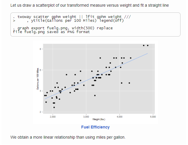
Let us read the fuel efficiency data that ships with Stata
sysuse auto, clear
To study how fuel efficiency depends on weight it is useful to transform
the dependent variable from “miles per gallon” to “gallons per 100
miles”
gen gphm = 100/mpg
We then obtain a fairly linear relationship
twoway scatter gphm weight || lfit gphm weight ///
ytitle(Gallons per 100 Miles) legend(off)
graph export auto.png, width(500) replace
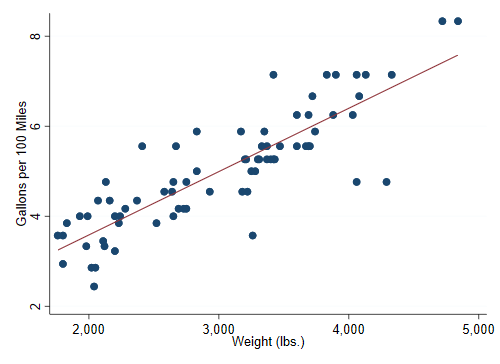
The regression equation estimated by OLS is
regress gphm weight
Thus, a car that weighs 1,000 pounds more than another requires on
average an extra 1.4 gallons to travel 100 miles.
That’s all for now!Saving the file as auto.stmd and running markstat using auto generates the web page shown at data.princeton.edu/stata/markdown/auto, with a screen capture shown in Figure 1.
Screen Capture of auto.html
The markstat command extracts the Markdown and Stata code into separate .md and .do files, taking care to mark where the code blocks came from. It then runs the Markdown code through an external program called Pandoc, runs the do file through Stata, and then weaves all the output together into a beautiful web page.
There are options to generate a PDF file instead of HTML, and to use the MathJax library to render equations on a web page. But before I explain these options let me tell you a bit about Markdown and Pandoc.
Markdown is a lightweight markup language invented by John Gruber. It is easy to write and, more importantly, it was designed to be readable “as is”, without intrusive markings. Yet it can easily be converted into valid HTML or PDF.
This section is a quick introduction to Markdown. Please refer to Gruber (2004)’s (2004) Markdown: Basics for more information. There is an ongoing effort to standardize Common Markdown, with reference implementations in C and JavaScript, visit commonmark.org for details.
In Markdown you create a heading by “underlining” your text using === for level 1 and --- for level 2, as we did in our example. One can also define headings at levels one to six by starting a line with one to six hashmarks, as in ### A level 3 heading.
You define a paragraph break by leaving a blank line. If you need a line break, end the line with two or more spaces (which are hard to see :), or end the line with \.
To indicate emphasis using an italic style wrap the text with one star or underscore, as in *italic* or _italic_. For strong emphasis using a bold font wrap the text with two stars or underscores, as in **bold** or __bold__. For a monospace font suitable for code wrap the text in backticks, typing `regress` to refer to the regress command.
Create a list by starting a line with *, +, or - for a bulleted/unordered list or 1. for a numbered/ordered list. You add items to a list by starting a line with the same symbol or with a number. Items in ordered lists are numbered consecutively regardless of which numbers you use. To end the list you enter a blank line.
You can link to another document by putting the anchor in square brackets and the link in parentheses, as in [GR’s website](http://data.princeton.edu).
To link to an image start with a bang, type a title in square brackets and the source of the image in parenthesis. For example .
An important feature of Markdown is that you can include HTML if you wish. For example we could have coded the image as <img src=auto.png/>, or a line break as <br/>. This is not recommended if the aim is to generate a PDF document.
To convert Markdown to HTML (or other formats) you need a document converter. I find that Pandoc works very well and is easy to install, with binaries for Linux, Mac and Windows, so that’s what we’ll use. Please visit pandoc.org/installing to download and install the program, unless of course it is already installed in your system.
To tell Stata where Pandoc was installed we use the whereis command, available from the SSC archive, just type ssc install whereis. This command maintains a registry of ancillary programs. To register the location of Pandoc you type in Stata
whereis pandoc full-path-to-pandoc-executablewhere the path should be quoted if it contains spaces.
For example on a Mac the full path may be /usr/local/bin/pandoc and on a Windows system it may be "c:\program files (x86)\pandoc\pandoc.exe", but of course the location in your system may be different. If you need assistance finding the location of Pandoc try help whereis and read the section “Tips for Users”, which notes how you can use the Unix commands which and whereis or the Windows command where to help locate the file.
Subsequent calls to whereis pandoc return the registered location, which is how markstat can find it.
Pandoc implements several extensions to Markdown, please refer to John MacFarlane’s (2006) Pandoc User’s Guide for details. For example the use of \ to force a line break is a Pandoc extension.
Another extension of note is that Pandoc will use the image title or alt-text, as specified in square brackets, to generate a caption for the figure. This means that your Stata code for generating the graph should probably not contain a title. Alternatively, you may leave the alt-text blank, or turn off captioning by ensuring that the image is not a separate paragraph, which you do by adding a backslash at the end of the line, as in \.
The syntax of the markstat command is quite simple:
markstat using filename [, pdf mathjax strict]The input file should have extension .stmd, which is short for Stata Markdown, and as usual with Stata commands it can be omitted. The sample file is called auto.stmd in my system, and I ran it by typing markstat using auto.
If all you want to do is generate HTML and your document does not include mathematical equations you don’t need any of the options, so I’ll provide only a brief summary here, leaving details to later sections. This also means that if you downloaded Pandoc and registered it with whereis you are now ready to run markstat.
The pdf option is used to generate a PDF document, which is done by first generating LaTeX, so it requires additional tooling as explained in §10.
The mathjax option is used to include inline and display math in a web page using the MathJax JavaScript library, see §7. The option is ignored for PDF output.
The strict option has to do with how we separate Markdown and Stata code. The “one tab or four spaces” rule is very simple and supports clean documents, but precludes some advanced Markdown options. The strict syntax uses code fences for maximum flexibility, and is described in §11.
The first thing the command does is tangle the file, extracting the Markdown and Stata blocks into separate files, which have the same name as the input file with extensions .md and .do, respectively.
The Markdown file has all Stata code removed, leaving placeholders of the form {{n}} for the n-th code chunk, which is why you should not use double braces as part of your annotations. But then, who does?
The command will try to convert this file to HTML or LaTeX using Pandoc, producing a file with the same name as the input and extension .pdx. This is a regular HTML or LaTeX file, but has a custom extension to distinguish it from the file that will incorporate Stata output later in the pipeline.
The Stata do file has all annotations removed. Instead it has comments of the form //_n to mark the start of the n-th code chunk and //_^ to mark the end of the last chunk, so please avoid this pattern in your own comments.
The next thing the command does is run this file through Stata. If something goes wrong you will see the reason in the results window. The output of this step is a log file in SMCL format, with .smcl extension.
The command then weaves the Markdown and Stata output files, taking care to insert the output in the appropriate places in the narrative as indicated by the placeholders. This produces a file with the same name as the input file and extension .html for HTML and .tex for LaTeX.
If you are generating HTML you are done. Generating a PDF document requires an extra step, running pdflatex to convert the LaTeX file to PDF, which markstat does by running an external program and using a Stata LaTeX package as described below.
Finally markstat issues the Stata command view browse to show the final document in your default web browser or Acrobat reader.
If your Stata program produced graphs and you generated HTML, the resulting file will not be self-contained because all it will have are links to the images, which will reside in your computer’s hard drive. If you were to email the file to a colleague it would be missing the images.
The bundle command, also available from the SSC archive, provides a solution. This command takes as input the name of an HTML file, goes through the code, and each time it finds a link to an image in PNG format it grabs the image file, encodes it as text using the same base 64 encoding as email attachments, and rewrites the image link to include the encoded image as URI data. By default the output file has the same name as the input with -b appended to indicate that it is a bundle, but there is an option to specify a different name.
For example to turn our fuel efficiency example into a self-contained web page we could use
bundle using autoThis will read auto.html and write auto-b.html with the image bundled in.
Another way to include images is to save the HTML file as PDF, which browsers such as Chrome will do for you. Yet another way is to read the HTML file into Word, which does a reasonably good job of parsing the code, and then save it as PDF. Still another way is to generate PDF instead of HTML, as explained in §10 below, as that will embed the images automatically.
Pandoc will take any text between dollar signs as a LaTeX formula, so you may write a regression model as $y = \alpha + \beta x + e$. Exactly how the equation is rendered depends on the type of output you are generating and the options in effect.
If you are generating HTML, Pandoc will render the equation as well as possible using Unicode characters. This is often all you need for simple equations. A more general solution is to use MathJax, which is enabled by markstat’s mathjax option.
MathJax is a Javascript library that can render LaTeX formulas in an HTML page with excellent results. Pandoc will let you use single dollar signs for inline math and double dollar signs for display math, just as you would in a LaTeX document, and will translate them to \( and \) for inline equations and \[ and \] for display equations, which is what MathJax prefers.
Pandoc will also make sure that the HTML file includes a link to the MathJax script using their content distribution network (CDN). Please visit MathJax.org for more information.
If you are generating PDF via LaTeX you can use single and double dollar signs too, and the inline and display math will be rendered natively by LaTeX.
When typing inline math make sure that there is no space between the equation and the opening or closing dollar signs. For example $ y = \alpha + \beta x + e $ will not work. For display math you can include the entire expression in one line using double dollar signs, but you can also display it as
$$
    y = \alpha + \beta x + e
$$
which I think improves readability. I found that I tend to indent the math in display equations, and of course I wouldn’t want it to be mistaken for Stata code under the “one tab or four spaces” rule, so markstat will suspend that rule inside display math, provided the double dollar signs are the only text in the opening and closing lines.
By the way the code above renders in PDF as
y = α + βx + e
Try generating HTML with and without the MathJax option to see what works for you.
Pandoc has an option to include a document’s title, author and date as metadata. All you do is begin the document with three lines that start with a % symbol and contain the relevant information:
% Stata Markdown
% Your Name Here
% 26 October 2016
In LaTeX this information will populate the title, author and date macros before generating the title page. In HTML it will appear as both metatada and as headings at levels 1, 2 and 3 at the start of the document.
To omit the title, author or date leave the line blank except for the %. If the title is too long you may continue on extra lines, provided you start them with a space. Multiple authors may be listed separated by semi-colons and/or on continuation lines. The date may be generated using inline code as noted in §12.
Alternatively, you may use the YAML format to enter the metadata. See the User’s Guide (MacFarlane 2006) for more information.
The markstat command comes with a Cascading Style Sheet (CSS) file that contains styles to be used in HTML output. The file has rules for headings, text, and of course Stata input and output blocks. It also provides styles for Pandoc-generated items such as metadata, figure environments, and figure captions. The CSS file is called markstat.css, will be saved in the ado path when the command is installed, and will be injected in the output when you generate HTML, so no external links are needed.
It is possible to customize the styles by using your own set of rules. All you have to do is define a CSS file and save it as markstat.css in the current directory, which is searched before the system directories. This setup also allows you to have a different style file for each project; you just use different folders, each with its own CSS file. The best way to get started is by editing the standard style.
All Stata input and output is rendered in HTML as preformatted text using a <pre> tag with class stata, with a light grey background and a border, both easily changed. The horizontal and vertical rules, corners, crossings and T-junctions typical of Stata output are rendered using Unicode versions of the original IBM drawing characters. I get best results specifying a Lucida Console font on Windows and just trusting the browser to pick a monospace font otherwise, with the line-height equal to the font-size. I recommend you keep these settings.
The simplest way to generate PDF output is to first generate HTML and then have your browser save the file as PDF, or read the file into Word and save it as PDF, as noted at the end of §6 in the context of bundling figures. This may be all you need.
For superior results, however, there is no substitute for first generating LaTeX and then converting that to PDF, which is what the pdf option does. The good news is that you don’t need to learn LaTeX, as you can author your annotations in Markdown, which is much easier.
Unfortunately this option requires additional tooling, as you need to have access to a LaTeX-to-PDF converter, which will usually be part of a TeX installation such as MiKTeX on Windows, MacTeX on Mac OS X, or TeX Live on Unix. If you are not a LaTeX user you will need to download one of these distributions.
You then use the whereis command introduced earlier to let markstat know where to find pdflatex, typing in Stata
whereis pdflatex full-path-to-pdflatex-executablesubstituting, of course, the path in your system. On a Windows system this may be c:\Program Files (x86)\MikTeX 2.9\mixtex\bin\pdflatex.exe, and on a Mac it might be /usr/local/texlive/2015/bin/x86_64-darwin/pdflatex, but of course the location in you system may differ. Type help whereis for tips locating the file.
You also need a Stata package used to render Stata logs in LaTeX. The file is called stata.sty and is available from the Stata Journal. There is a command called sjlatex that will install all journal files, but we only need stata.sty, which can be downloaded from http://www.stata-journal/production/sjlatex/stata.sty. The file may be in the current directory, but it is more convenient to copy it to your local TeX installation and then update the TeX filename database, so the package is always available. Having access to a local TeX guru may be invaluable at this stage.
Once these two tooling requirements have been satisfied, using the pdf option will cause markstat to tangle the input, run Pandoc to generate LaTeX from the Markdown code, run the Stata do file, ask Stata to convert the SMCL log to TeX via the log texman command, weave the outputs into a single LaTeX file, run pdflatex, and then display the PDF file in Acrobat Reader via Stata’s view browse command.
On some systems pdflatex may not be able to write to the PDF file if it is open in Adobe Reader, and will stop and ask for another file name. The workaround is to close the reader, and then press enter in the converter window so it can resume its work. Even better is to make a habit of closing the PDF file before re-running the markstat command. There are other PDF viewers that do not lock the file, but I prefer to follow Stata defaults.
If you are generating a PDF file the images will have been embedded automatically. For best results, however, your graph export command should probably generate images in PDF rather than PNG format. PDF uses a vector format, essentially instructions for drawing the image, and scales better than PNG, a raster format consisting basically of a matrix of pixels of different colors.
The decision to define a Stata block by indenting each line of code one tab or four spaces produces very clean-looking input files which happen to be legal Markdown code.
There is, however, a small problem. The Common Markdown specification allows a list item to have more than one paragraph and/or include nested lists, with the subsequent paragraphs or lists indented one tab or four spaces. As a result our simple rule will mistake those lines for Stata commands. The workaround is simple: stick to simple lists, or read on for an alternative.
There is also an issue if you want to include verbatim blocks that are not intended to be run through Stata, but this problem can be solved by using code fences, lines with three or more backticks or tildes inserted before and after a block of code. The markstat parser will not treat fenced code as Stata even if indented.
A more general solution is to use code fences for Stata blocks themselves, coding
```{s}
   // Stata commands here
```
This makes the block clear and unambiguous, with the {s} indicating that the code is to be run through Stata. It also allows multiparagraph list items and nested lists. But it does make the input file look a bit more cluttered; which is why, in the interest of readability, this is not the default setting.
The strict option of the markstat command turns on Stata code fences, with the option to omit the braces, so a Stata block can start with the line ```{s} or just ```s and end with the line ```. For example the last part of our fuel efficiency example could be coded in strict mode as follows:
The regression equation estimated by OLS is

```s
    regress gphm weight
```

Thus, a car that weighs 1,000 pounds more than another requires on
average an extra 1.4 gallons to travel 100 miles.
When this option is in effect, indented blocks without Stata code fences will be treated as Markdown rather than Stata code, and therefore will be passed on to Pandoc for processing.
Code inside Stata fences may be indented to improve readability, as I did in the above example, and markstat will remove one level of indentation (if present) when generating the do file. Pandoc requires that fenced code blocks be separated from surrounding text by blank lines, but markstat makes those optional for Stata code blocks.
Using strict code blocks also allows you to turn off echoing the Stata commands in a code chunk, which you do by coding the opening fence
as ```{s/} with abbreviation ```s/. Examples are provided in §13 and §14.
This option may seem to run against the aim of full reproducibility of results, but it may be desirable when generating dynamic reports, where the commands themselves are of secondary interest and may safely be relegated to the .stmd file, which as noted in the introduction remains as a complete reproducible record of how everything was done.
There is no chunk option for suppressing Stata output because this can always be achieved using the quietly prefix. I imagine one might combine suppressing both input and output and running a script only for its side effects, which brings us to the next topic.
Sometimes your annotations need to quote results. For example after running a regression you may want to quote the value of R-squared. You could, of course, type something like “The proportion of variance explained or R-squared can be read from the output as 0.0077 or less than one percent.”
But that risks transcription errors. We know that Stata stores R-squared as e(r2) and it would be nice to access the stored result. One can always add display e(r2) to a code block, but the result would not be spliced with the text.
Enter inline code, which lets you quote results using an optional format and an expression with the following syntax
`s [fmt] expression`The code will extract the optional format and expression, run it through Stata using a display command, and then splice the output inline with the text.
For example we could say R-squared is `s e(r2)`, but you may not want to display R-squared to 8 decimal places, so try R-squared is `s%5.3f e(r2)` instead.
This feature is intended for short text. Inline code should not span multiple lines, but a line of Markdown text may include multiple inline expressions. The markstat command will retrieve just one line of output per expression.
Here is an example quoting an estimated coefficient dynamically:
Let us regress gallons per 100 miles on weight

    regress gphm weight

A car that weights 1,000 pounds more than another will use on average an
extra `s %5.2f 1000*_b[weight]` gallons to travel 100 miles.
The output from markstat with the pdf option will render as follows:
Let us regress gallons per 100 miles on weight
. regress gphm weight

      Source │       SS           df       MS      Number of obs   =        74
─────────────┼──────────────────────────────────   F(1, 72)        =    194.71
       Model │  87.2964969         1  87.2964969   Prob > F        =    0.0000
    Residual │  32.2797639        72  .448330054   R-squared       =    0.7300
─────────────┼──────────────────────────────────   Adj R-squared   =    0.7263
       Total │  119.576261        73  1.63803097   Root MSE        =    .66957

─────────────┬────────────────────────────────────────────────────────────────
        gphm │      Coef.   Std. Err.      t    P>|t|     [95% Conf. Interval]
─────────────┼────────────────────────────────────────────────────────────────
      weight │    .001407   .0001008    13.95   0.000      .001206    .0016081
       _cons │   .7707669   .3142571     2.45   0.017     .1443069    1.397227
─────────────┴────────────────────────────────────────────────────────────────
A car that weights 1,000 pounds more than another will use on average an extra 1.41 gallons to travel 100 miles.
It is possible to style the output of inline expressions as code by using double backticks. For example in the fuel efficiency data we could state that the variance was estimated using the ``s e(vce)`` method, which in this case would render as “the ols method”, with ols in a monospace font.
Inline code may be inserted anywhere in Markdown, including the metadata. For example the date line may read % `s c(current_date)` to insert the current date as provided by Stata’s c-class.
Finally, inline code may include macro evaluations and/or compound quotes. Just keep in mind that Stata macros use an opening backtick and a closing single quote, whereas inline code uses opening and closing backticks, which is how the parser can distinguish them. We’ll see an example in the next section.
On occasion your narrative may need to include a table of results. Markdown does not have a syntax for tables, relying on HMLM markup instead, but Pandoc provides a simple syntax extension, best described through an example.
Here is code for a table showing average fuel efficiency in gallons per 100 miles for foreign and domestic cars, before and after adjusting for weight.
Car Type      Unadjusted    Adjusted
----------  ------------  ----------
Foreign           4.31         5.46
Domestic          5.32         4.83
Basically you line up the columns yourself. Text alignment is determined by the position of the header relative to the “underlining” below it. Our first column is left-aligned and the other two are right-aligned.
While pleasantly simple, this syntax will not work if we have inline code, as the expressions, their placeholders, and the final output may all have different widths. Fortunately, Pandoc has an alternative syntax, pipe tables, where columns are separated by the pipe character | and alignment is indicated by the placing of a colon in the header underlining. The previous example would look as follows:
| Car Type | Unadjusted |  Adjusted |
|:---------|-----------:|----------:|
| Foreign  |     4.31   |    5.46   |
| Domestic |     5.32   |    4.83   |
Now we can make the table truly dynamic. We regress gallons per 100 miles on the indicator of foreign cars and store the coefficients in a matrix. We then compute the mean weight and store it for later use. Finally we add weight to the regression model. To keep the code short I stored the baseline prediction (domestic cars of average weight) in a scalar. Because we want to display all results to just two decimal places we store a common format in a macro. This is also a good candidate for hiding all commands.
```s/
    quietly reg gphm foreign
    mat b = e(b)
    quietly sum weight
    scalar mw = r(mean)
    quietly reg gphm weight foreign
    scalar dom = _b[_cons] + _b[weight] * mw
    local f %6.2f
```
We are then ready to layout the table using inline code as shown below. I lined up the pipe characters to improve readability, but that is not required, and in any case it would no longer hold after markstat splices the actual results.
| Car Type | Unadjusted            | Adjusted                  |
|:---------|----------------------:|--------------------------:|
| Foreign  | `s `f' b[1,1]+b[1,2]` | `s `f' dom + _b[foreign]` |
| Domestic | `s `f' b[1,2]`        | `s `f' dom`               |
This code with the pdf and strict options renders the following table:
| Car Type | Unadjusted | Adjusted |
|---|---|---|
| Foreign | 4.31 | 5.46 |
| Domestic | 5.32 | 4.83 |
Foreign cars use less fuel than domestic cars but are also lighter; when we compare cars with the same weight, the imports use about six-tenths of a gallon more per 100 miles than comparable domestic cars.
I mentioned in the introduction commands aimed at producing publication-quality tables, some of which have options to export results to LaTeX, Word or Excel. As long as they also produce standard Stata output, however, they can be used with markstat.
I will illustrate this possibility using Jann’s (2007) esttab, a nice wrapper for estout that works with eststo to store equation results. The following Stata Markdown script fits two models to the fuel efficiency data and compares them side-by-side. We use the strict syntax and suppress command echoing, to show what a dynamic summary report might look like:
The table below shows estimated differences in fuel efficiency between
foreign and domestic cars with and without adjustment for weight, using
gallons per 100 miles as the outcome.

````s/
    eststo clear
    quietly eststo: regress gphm foreign
    quietly eststo:regress gphm foreign weight
    esttab
```

We see that on average foreign cars are more economical, but
if we adjust for weight they are less fuel efficient, using
`s %3.1f _b[foreign]` gallons *more* instead of one gallon
*less* per 100 miles.
Running this code with the pdf and strict options produces the following output:
The table below shows estimated differences in fuel efficiency between foreign and domestic cars with and without adjustment for weight, using gallons per 100 miles as the outcome.
────────────────────────────────────────────
                      (1)             (2)
                     gphm            gphm
────────────────────────────────────────────
foreign            -1.005**         0.622**
                  (-3.29)          (3.11)

weight                            0.00163***
                                  (13.74)

_cons               5.318***      -0.0735
                  (31.92)         (-0.18)
────────────────────────────────────────────
N                      74              74
────────────────────────────────────────────
t statistics in parentheses
* p<0.05, ** p<0.01, *** p<0.001
We see that on average foreign cars are more economical, but if we adjust for weight they are less fuel efficient, using 0.6 gallons more instead of one gallon less per 100 miles.
The estout command can also produce HTML and LaTeX tables, as does tabout (Watson 2016). It is possible to include these tables in the output as long as they are in the target language, and I provide examples online.
Rising (2016) has a nice review of current tools for producing dynamic documents in Stata. I believe markstat fills all the requirements he mentions for teaching and research, such as including or hiding commands and/or results, inserting graphs, and quoting results in the narrative, and has an important advantage over other tools in the simplicity of the single-file input script.
In fact the overriding concern in the design of the markstat command has been simplicity. I wanted the input file to be easy to write and, just as importantly, easy to read, much in the spirit of Markdown itself, with minimal intrusion from the need to distinguish Stata and Markdown code.
I rely on a simple “one tab or four spaces” indentation rule to produce clean input, but allow fenced blocks for maximum flexibility, as well as inline code for quoting results. All the inline or block code is plain Stata, without the need for special commands. And everything outside those elements is plain Markdown.
I modeled the output on Stata’s own documentation and this journal. The task was made easier, at least when generating PDF output, by using the same LaTeX style. The HTML output tries to live up to that standard by taking advantage of Unicode to render horizontal and vertical rules using the original IBM drawing characters, which are available in modern monospace fonts.
To facilitate troubleshooting I make minimal use of temporary files, keeping all important pieces around. As noted earlier the tangle step generates a standard Stata do file, and if something goes wrong there you will soon see the cause in the results window.
The command also generates a standard Markdown file, but if something goes wrong with Pandoc it may be harder to detect the problem because the shell will have closed. My advice here is to run Pandoc from a terminal or command window. Producing PDF is harder because it requires LaTeX, and my troubleshooting advice again is to run pdflatex directly on a console to see what went wrong.
I have assumed that the user will be writing Stata code and Markdown annotations at the same time, but as a reviewer noted it is also possible to convert existing do files into Stata Markdown scripts, indenting the code and rewriting or expanding the comments using Markdown syntax.
The Stata Markdown section of my website has installation tips and a growing collection of examples. It will also include answers to frequently-asked questions, see http://data.princeton.edu/stata/markdown.
I am very grateful to an anonymous reviewer for thoughtful comments that improved the presentation and its relevance to applied researchers pursuing reproducible research.
Allaire, JJ, Joe Cheng, Yihui Xie, Jonathan McPherson, Winston Chang, Jeff Allen, Hadled Wickman, Aron Atkins, and Rob Hyndman. 2016. “Dynamic Documents for R.” http://rmarkdown.rstudio.com.
Barba, Lorena A. 2016. “The Hard Road to Reproducibility.” Science 354 (6308). http://science.sciencemag.org/content/354/6308/142.
Gallup, John Luke. 1999. “outreg: Stata Module to Write Estimation Tables to a Word or Tex File.” https://ideas.repec.org/c/boc/bocode/s375201.html.
Gangrud, Christopher. 2015. Reproducible Research with R and RStudio. 2nd ed. Chapman & Hall/CRC.
Gruber, John. 2004. “Markdown: Basics.” https://daringfireball.net/projects/markdown/basics/.
Haghish, E. F. 2016. “markdoc: Literate Programming in Stata.” Stata Journal 16 (4): 964–88.
Hemken, Doug. 2015. “Stata and R Markdown (Windows).” http://goo.gl/QdrVn5.
Jann, Ben. 2005. “Making Regression Tables from Stored Estimates.” Stata Journal 5 (3): 288–308.
———. 2007. “Making Regression Tables Simplified.” Stata Journal 7 (2): 227–44.
———. 2016a. “Creating Latex Documents from Within Stata Using texdoc.” Stata Journal 16 (2): 245–63.
———. 2016b. “webdoc: Stata Module to Create a HTML or Markdown Document Including Stata Output.” http://ideas.repec.org/c/boc/bocode/s458209.html.
Knuth, Donald. 1992. Literate Programming. Stanford, CA: CSLI Lecture Notes.
Leisch, F. 2002. “Sweave: Dynamic Generation of Statistical Reports Using Literate Data Analysis.” In Compstat 2002. Proceedings in Computational Statistics, edited by Wolfgang Härdle and Bernd Rönz, 575–80. Physika Verlag, Heidelberg, Germany.
MacFarlane, John. 2006. “Pandoc User’s Guide.” http://pandoc.org/MANUAL.pdf.
Peng, Roger D. 2009. “Reproducible Research and Biostatistics.” Biostatistics 10 (3): 405–8.
Quintó, Llorenc, Sergi Sanz, Elisa De Lazzari, and John J. Aponte. 2012. “HTML Output in Stata.” Stata Journal 12 (4): 702–17. http://www.stata-journal.com/article.html?article=dm0066.
Rising, Bill. 2016. “Dynamic Documents in Stata: Many Routes to the Same Goal.” http://www.sugm.net.au/docs/papers2016/Rising.pdf.
Rossini, A. J. 2001. “Literate Statistical Practice.” In DSC 2001. Proceedings of the 2nd International Workshop on Distributed Statistical Computing, edited by K. Hornick and F. Leisch. http://www.R-project.org/conferences/DSC-2001.
Wada, Roy. 2005. “outreg2: Stata Module to Arrange Regression Outputs into an Illustrative Table.” https://ideas.repec.org/c/boc/bocode/s456416.html.
Watson, Ian. 2016. “Publication Quality Tables in Stata. User Guide for tabout. Version 3.” http://tabout.net.au/downloads/tabout_user_guide.pdf.
Xie, Yihui. 2016. Dynamic Documents with R and Knitr. 2nd ed. Chapman & Hall/CRC.