---
title: Cox Regression
author: Germán Rodríguez
date: 12 December 2017
header-includes:
-
-
-
-
---
::: {.container}
We continue our analysis of the Gehan data by fitting a proportional hazards
model. This is the same dataset used as an example in Cox's original paper:
Cox, D.R. (1972) Regression Models and Life tables, (with discussion) *Journal
of the Royal Statistical Society*, __34__: 187–220.
```r/
# set up a couple of libraries and a function to ggfy generic plots
library(dplyr)
library(ggplot2)
ggfy <- function(obj, ...) {
p <- par(c("mar","mgp","tck","cex"))
par(mar=c(3,3,2,1), mgp=c(2,.7,0), tck=-.01, cex = 0.7)
plot(obj, ...)
u <- par("usr")
rect(u[1], u[3], u[2], u[4], col="#ebebeb", border="#ebebeb")
grid(lty=1, col="white")
par(new=TRUE)
plot(obj, axes=FALSE, ...)
par(p)
invisible(NULL)
}
```
The first task is to read [and `stset`]{.stata} the data.
I also create a dummy variable for `treated`.
```s
infile group weeks relapse using ///
https://grodri.github.io/datasets/gehan.raw, clear
gen treated = group == 2
stset weeks, failure(relapse)
```
```r
gehan <- read.table("https://grodri.github.io/datasets/gehan.dat")
names(gehan)
summarize(gehan, events = sum(relapse), exposure = sum(weeks))
gehan <- mutate(gehan, treated = as.numeric(group == "treated"))
```
Here's a run fitting a Cox model with all the defaults
```s
stcox treated
di _b[treated]
```
```r
library(survival)
cm <- coxph(Surv(weeks, relapse) ~ treated, data = gehan)
cm
```
[Stata reports hazard ratios unless you specify the option `nohr`.]{.stata}
[R reports log-relative risks, but also exponentiates the coefficients to obtain
hazard ratios.]{.r}
We see that the treatment reduced the risk of relapse by almost 80% at any
duration.
## Handling Ties
There are various options for handling ties. Cox's original proposal relies on
the discrete partial likelihood. A closely-related alternative due to
Kalbfleisch and Prentice uses the marginal likelihood of the ranks. Both methods
are computationally intensive. A good fast approximation is due to Efron, and a
simpler and faster, though somewhat less accurate, method is due to Breslow and
Peto. See the notes for details.
In terms of our software,
[Stata implements all four using the options `exactp`, `exactm`, `efron` and
`breslow`. The default is `breslow` but I recommend you always use `efron`.]{.stata}
[R implements all but the marginal likelihood, using the argument `ties` with
possible values "efron", "breslow", and "exact".]{.r}
Let us compare them all.
```s
estimates store breslow
quietly stcox treated, efron
estimates store efron
quietly stcox treated, exactm
estimates store exactm
quietly stcox treated, exactp
estimates store exactp
estimates table breslow efron exactm exactp
```
```r
cmb <- coxph(Surv(weeks, relapse) ~ treated, data = gehan, ties="breslow")
cmp <- coxph(Surv(weeks, relapse) ~ treated, data = gehan, ties="exact")
data.frame(breslow = coef(cmb), efron = coef(cm), exact = coef(cmp))
```
As you can see, Efron's approximation is closer to the exact partial likelihood
than Breslow's. [The marginal likelihood is even closer.]{.stata}
Cox reported a log-likelihood of -1.65 in his paper, which he obtained by
evaluating the likelihood in a grid of points. The more exact calculations here
yield -1.63, so he did pretty well by hand (see page 197 in the paper).
## Proportionality of Hazards
One way to test proportionality of hazards is to introduce interactions with
duration. In his original paper Cox tried a linear interaction with time.
We will do the same, except that he worked with *t - 10* to achieve more
orthogonality and we will use *t*.
### Stata's tvc() and texp()
Stata makes it very easy to introduce interactions with time by providing two
options:
1. `tvc(varlist)`, to specify the variable(s) we want to interact with time, and
1. `texp(expression)`, to specify a function of time `_t`, typically just time,
`texp(_t)`, or log-time, `texp(log(_t)`.
Stata will then create a variable equal to the product of the variable specified
in `tvc()` by the time expression specified in `texp()` and add it to the model.
Let us use this technique to interact treatment and time
```s
stcox treated, tvc(treated) texp(_t) efron
```
We see that there's no evidence that the treatment effect changes linearly with
time. BTW we didn't really have to specify `texp(_t)` because that's the default.
Another possibility is to allow different treatment effects at early and late
durations, say before and after 10 weeks.
This is easily done by changing the time expression:
```s
stcox treated, tvc(treated) texp(_t > 10) efron
```
The point estimates indicate a 73% reduction in risk in the first ten weeks and
an additional 44% reduction after ten weeks, for a total of 85% in the later
period. However, the difference in treatment effects between the two periods is
not significant.
### Splitting at Failures
Because only times with observed failures contribute to the partial likelihood,
we can introduce arbitrary interactions by splitting the data at each failure
time. As a sanity check, we verify that we obtain the same estimate as before
```s
gen id = _n // need an id variable to split
streset, id(id)
stsplit , at(failures)
quietly stcox treated, efron
di _b[treated]
estimates store ph
```
```r
failure_times <- sort(unique(gehan$weeks[gehan$relapse]))
gehanx <- survSplit(gehan, cut = failure_times,
event = "relapse", start = "t0", end = "weeks")
coef(coxph(Surv(t0, weeks, relapse) ~ treated, data=gehanx))
```
We now introduce a linear interaction with time using our dummy variable for
`treated`.
[(You could specify the model as `group * t0`. R will omit `t0` because it is
implicit in the baseline hazard and complain that the model matrix is singular,
but the results will be correct. My approach is a bit cleaner.)]{.r}
```s
stcox treated c.treated#c._t, efron
lrtest ph .
stjoin // back to normal
```
```r
cmx <- coxph(Surv(t0, weeks, relapse) ~ treated + treated:weeks, data=gehanx)
summary(cmx)
c( logLik(cmx), logLik(cm))
```
We get a Wald test for the interaction term of z = 0.01 and
twice a difference in log-likelihoods of 0.00, so clearly there is
no evidence of an interaction between treatment and time at risk.
[Note that these are exactly the same results we got with `tvc()` and `texp()`]{.stata}
## Split at 10
As an alternative we could allow different treatment effects before and after
10 weeks. We could use the current dataset, but all we really need is to split
at 10, so we'll do just that:
```s
stsplit dur, at(10)
quietly stcox treated, efron // so we can do lrtest
estimates store ph
gen after10 = dur == 10
stcox treated c.treated#c.after10, efron
lrtest ph .
drop dur after10
stjoin
```
```r
gehan10 <- survSplit(gehan, cut = 10,
event = "relapse", start = "t0", end = "weeks") %>%
mutate(after10 = as.numeric(t0 == 10),
treated = as.numeric(group == "treated"))
cm10 <- coxph(Surv(t0, weeks, relapse) ~ treated + treated:after10,
data=gehan10)
summary(cm10)
chisq <- 2*(logLik(cm10) - logLik(cm)); chisq
```
The Wald test now yields -0.73 (a chi-squared of 0.53),
and the likelihood ratio test concurs, with a chi-squared of 0.54 on one d.f.
The risk ratio is a bit larger after 10 weeks, but the difference is still
not significant.
[Note that these are exactly the same results we got with `tvc()` and
`texp()`.]{.stata}
## Schoenfeld Residuals
Another way to check for proportionality of hazards is to use Schoenfeld
residuals (and their scaled counterparts). You can obtain an overall test using
the Schoenfeld residuals, or a variable-by-variable test based on the scaled
variant. In this case with just one predictor there is only one test, but we'll
see later an example with several predictors.
Stata and R offer several possible transformations of time for the test,
including a user-specified function, but chose different defaults.
In Stata the default is time, but one of the options is `km` for the Kaplan-Meier
estimate of overall survival.
In R the default transform is "km" for the K-M estimate, but one of the options
is "identity".
```s
quietly stcox treated, efron
estat phtest
```
```r
zph <- cox.zph(cm , transform="identity")
zph
```
The test shows that there is no evidence against the proportional hazards
assumption. If there had been, we could get a hint of the nature of the time
dependence by plotting the (scaled) residuals against time and using a smoother
to glean the trend, if any.
[In R the `cox.zph` class has a `plot()` method which uses a spline smoother.
I specified `df=2` because of the small sample size.]{.r}
```s
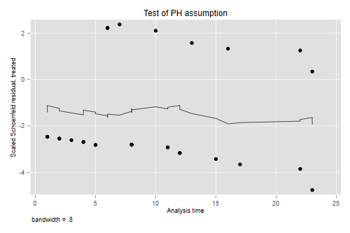
estat phtest, plot(treated)
graph export phplot.png, width(500) replace
```
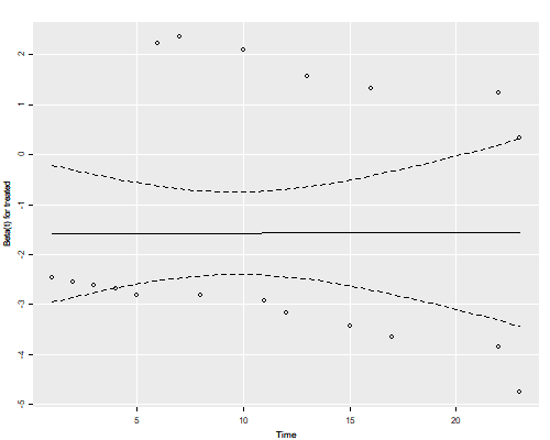
```r
png("phplotr.png", width=500, height=400)
ggfy(zph, df=2)
dev.off()
```
{.img-responsive .img-center .stata}
{.img-responsive .img-center .r}
The residuals show no time trend at all, showing that the treatment hazard ratio
is fairly constant over time. (We will confirm this result below with a plot of
cumulative hazards that provides more direct evidence.)
## Baseline Survival
The emphasis in the Cox model is on hazard ratios, but one can calculate a
Kaplan-Meier or a Nelson-Aalen estimate of the baseline survival, as shown in
the notes. The baseline is defined as the case where all covariate values are
zero, and this may not make sense in your data. A popular alternative is to
estimate the "baseline" at average values of all covariates. In our case a much
better approach is to estimate and plot the estimated survival functions for the
two groups.
[Stata makes this very easy via the `stcurve` command]{.stata}
```s
stcurve, surv at(treated=0) at(treated=1)
```
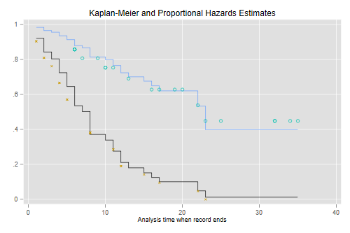
It is instructive to compute these "by hand" and compare them with separate
Kaplan-Meier estimates for each group, which I will plot using different symbols
for treated and controls. The plots connect the point estimates using a step
function.
```s
predict S0, basesurv // control (not mean!)
gen S1 = S0^exp(_b[treated]) // treated
sts gen KM = s, by(treated) // two Kaplan-Meiers
twoway (scatter S0 _t, c(J) ms(none) sort) /// baseline
(scatter S1 _t , c(J) ms(none) sort) /// treated
(scatter KM _t if treated, msymbol(circle_hollow)) /// KM treated
(scatter KM _t if !treated, msymbol(X)) /// KM base
, legend(off) ///
title(Kaplan-Meier and Proportional Hazards Estimates)
graph export coxkm.png, width(500) replace
```
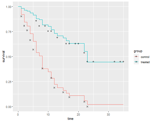
```r
sf <- survfit(cm, newdata=list(treated=c(1,0)))
km <- survfit(Surv(weeks, relapse) ~ treated, data=gehan)
dsf <- data.frame(time = rep(c(0,sf$time), 2),
survival = c(1, sf$surv[,1], 1, sf$surv[,2]),
group = factor(rep(c("treated","control"),
rep(length(sf$time) + 1,2))))
dkm <- data.frame(time = km$time,
survival = km$surv,
group = factor(rep(c("treated","control"),
km$strata)))
ggplot(dsf, aes(time, survival, color = group)) + geom_step() +
geom_point(data = dkm, aes(time, survival, shape=group),color="black") +
scale_shape_manual(values = c(1, 4))
ggsave("coxkmr.png", width=500/72, height=400/72, dpi=72)
```
{.img-responsive .img-center .stata}
{.img-responsive .img-center .r}
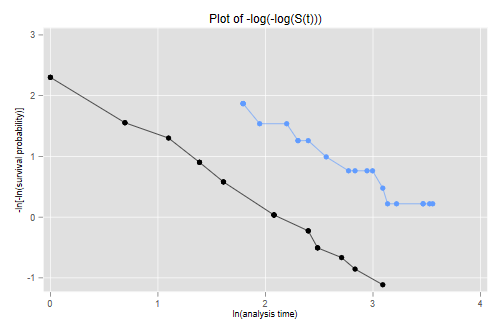
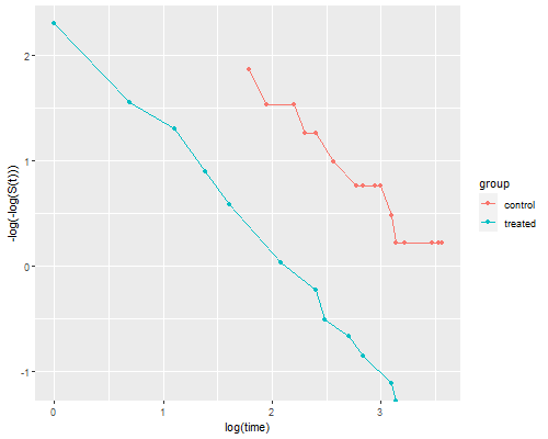
The figure looks just like Figure 1 in Cox's paper. If the purpose of the graph
is to check the proportional hazards assumption a much better alternative is to
plot the log-log transformation of the survival function, namely -log(-log(S(t)),
against log(t) for each group. Under the proportional hazards assumption the
resulting curves should be parallel. This plot is useful because the eye is much
better at judging whether curves are parallel than whether they are proportional.
```s
stphplot, by(treated) legend(off) title(Plot of -log(-log(S(t))))
graph export coxphplot.png, width(500) replace
```
```r
dkm <- mutate(dkm, lls = -log(-log(survival)))
ggplot(dkm, aes(log(time), lls, color=group)) + geom_point() +
geom_line() + ylab("-log(-log(S(t)))")
ggsave("coxphplotr.png", width=500/72, height=400/72, dpi=72)
```
{.img-responsive .img-center .stata}
{.img-responsive .img-center .r}
The two lines look quite parallel indeed.
:::