
Here’s an interesting example where fixed-effects gives a very different answer from OLS and random-effects models. The data come from Wooldridge’s text and concern state-level data on the percentage of births classified as low birth weight and the percentage of the population in the AFDC welfare program in 1987 and 1990. The data are available from the Stata website.
. use https://www.stata.com/data/jwooldridge/eacsap/lowbirth, clear
Here’s a regression of low birth weight on AFDC with a dummy for 1990 (time trends) and controls for log physicians per capita, log beds per capita, log per capita income, and log population.
. reg lowbrth d90 afdcprc lphypc lbedspc lpcinc lpopul

      Source │       SS           df       MS      Number of obs   =       100
─────────────┼──────────────────────────────────   F(6, 93)        =      5.19
       Model │  33.7710894         6   5.6285149   Prob > F        =    0.0001
    Residual │  100.834005        93  1.08423661   R-squared       =    0.2509
─────────────┼──────────────────────────────────   Adj R-squared   =    0.2026
       Total │  134.605095        99  1.35964742   Root MSE        =    1.0413

─────────────┬────────────────────────────────────────────────────────────────
     lowbrth │ Coefficient  Std. err.      t    P>|t|     [95% conf. interval]
─────────────┼────────────────────────────────────────────────────────────────
         d90 │   .5797136   .2761244     2.10   0.038     .0313853    1.128042
     afdcprc │   .0955932   .0921802     1.04   0.302    -.0874584    .2786448
      lphypc │   .3080648     .71546     0.43   0.668    -1.112697    1.728827
     lbedspc │   .2790041   .5130275     0.54   0.588    -.7397668    1.297775
      lpcinc │  -2.494685   .9783021    -2.55   0.012      -4.4374   -.5519711
      lpopul │    .739284   .7023191     1.05   0.295    -.6553826    2.133951
       _cons │   26.57786   7.158022     3.71   0.000     12.36344    40.79227
─────────────┴────────────────────────────────────────────────────────────────
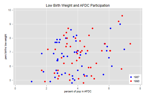
It seems as if AFDC has a pernicious effect on low birth weight: each percent in AFDC is associated with an extra 1/10-th of one percent with low birth weight. A scatterplot shows a positive correlation:
. twoway (scatter lowbrth afdcprc if year==1987, mcolor(blue) ) ///
>   (scatter lowbrth afdcprc if year==1990, mcolor(red)  ) , ///
>   legend( lab(1 "1987") lab(2 "1990") ring(0) pos(5) ) ///
>   title(Low Birth Weight and AFDC Participation)

.   graph export afdc1.png, width(500) replace
file afdc1.png saved as PNG format
Fitting a random-effects model improves things a bit. I first
encode the state abbreviation to have a numeric id
variable. For this dataset the results with xtreg and
mixed are a bit different. I report the results for
mixed, which agrees with R.
. encode stateabb, gen(stateid)

. mixed lowbrth d90 afdcprc lphypc lbedspc lpcinc lpopul || stateid:

Performing EM optimization ...

Performing gradient-based optimization:
Iteration 0:   log likelihood = -79.732599
Iteration 1:   log likelihood = -79.732599

Computing standard errors ...

Mixed-effects ML regression                     Number of obs     =        100
Group variable: stateid                         Number of groups  =         50
                                                Obs per group:
                                                              min =          2
                                                              avg =        2.0
                                                              max =          2
                                                Wald chi2(6)      =      24.39
Log likelihood = -79.732599                     Prob > chi2       =     0.0004

─────────────┬────────────────────────────────────────────────────────────────
     lowbrth │ Coefficient  Std. err.      z    P>|z|     [95% conf. interval]
─────────────┼────────────────────────────────────────────────────────────────
         d90 │    .506784   .1837357     2.76   0.006     .1466687    .8668994
     afdcprc │  -.0823577   .0778829    -1.06   0.290    -.2350054      .07029
      lphypc │   .2926323   .8293795     0.35   0.724    -1.332922    1.918186
     lbedspc │   .4291244   .5088063     0.84   0.399    -.5681176    1.426366
      lpcinc │  -1.681796   .9542535    -1.76   0.078    -3.552099    .1885062
      lpopul │   .7490035   .8004223     0.94   0.349    -.8197953    2.317802
       _cons │   20.12827   7.763454     2.59   0.010     4.912177    35.34436
─────────────┴────────────────────────────────────────────────────────────────

─────────────────────────────┬────────────────────────────────────────────────
  Random-effects parameters  │   Estimate   Std. err.     [95% conf. interval]
─────────────────────────────┼────────────────────────────────────────────────
stateid: Identity            │
                  var(_cons) │   1.035848   .2183906      .6852274    1.565875
─────────────────────────────┼────────────────────────────────────────────────
               var(Residual) │   .0394129   .0081434      .0262884    .0590896
─────────────────────────────┴────────────────────────────────────────────────
LR test vs. linear model: chibar2(01) = 125.15        Prob >= chibar2 = 0.0000

. estat icc

Residual intraclass correlation

─────────────────────────────┬────────────────────────────────────────────────
                       Level │        ICC   Std. err.     [95% conf. interval]
─────────────────────────────┼────────────────────────────────────────────────
                     stateid │   .9633458   .0108404      .9350615    .9795797
─────────────────────────────┴────────────────────────────────────────────────
The effect of AFDC is now negative, as we would expect, but not significant. The intra-state correlation over the two years is a remarkable 0.96; persistent state characteristics account for most of the variation in the percent with low birth weight after controlling for AFDC participation and all other variables.
Fitting a fixed-effects model gives much more reasonable results:
. xtreg lowbrth d90 afdcprc lphypc lbedspc lpcinc lpopul, i(stateid) fe

Fixed-effects (within) regression               Number of obs     =        100
Group variable: stateid                         Number of groups  =         50

R-squared:                                      Obs per group:
     Within  = 0.3839                                         min =          2
     Between = 0.1741                                         avg =        2.0
     Overall = 0.1679                                         max =          2

                                                F(6,44)           =       4.57
corr(u_i, Xb) = -0.9394                         Prob > F          =     0.0011

─────────────┬────────────────────────────────────────────────────────────────
     lowbrth │ Coefficient  Std. err.      t    P>|t|     [95% conf. interval]
─────────────┼────────────────────────────────────────────────────────────────
         d90 │   .1060158   .3090664     0.34   0.733    -.5168667    .7288983
     afdcprc │  -.1760763   .0903733    -1.95   0.058    -.3582116     .006059
      lphypc │   5.894509   2.816689     2.09   0.042     .2178452    11.57117
     lbedspc │  -1.576195   .8852111    -1.78   0.082    -3.360221    .2078308
      lpcinc │  -.8455268   1.356773    -0.62   0.536    -3.579924     1.88887
      lpopul │   3.441116   2.872175     1.20   0.237    -2.347372    9.229604
       _cons │    -4.0138   22.97888    -0.17   0.862    -50.32468    42.29708
─────────────┼────────────────────────────────────────────────────────────────
     sigma_u │  3.0975315
     sigma_e │  .18464547
         rho │  .99645917   (fraction of variance due to u_i)
─────────────┴────────────────────────────────────────────────────────────────
F test that all u_i=0: F(49, 44) = 59.46                     Prob > F = 0.0000
Now every percent increase in AFDC is associated with a decline of almost 2/10-th of a percentage point in low birth weight. The coefficient of log physicians per capita is highly suspect; this is due to high correlation with the other predictors, most notably the log of population. In fact once we have state fixed effects we don’t really need the other controls:
. xtreg   lowbrth d90 afdcprc, i(stateid) fe

Fixed-effects (within) regression               Number of obs     =        100
Group variable: stateid                         Number of groups  =         50

R-squared:                                      Obs per group:
     Within  = 0.2602                                         min =          2
     Between = 0.0948                                         avg =        2.0
     Overall = 0.0694                                         max =          2

                                                F(2,48)           =       8.44
corr(u_i, Xb) = -0.4366                         Prob > F          =     0.0007

─────────────┬────────────────────────────────────────────────────────────────
     lowbrth │ Coefficient  Std. err.      t    P>|t|     [95% conf. interval]
─────────────┼────────────────────────────────────────────────────────────────
         d90 │   .2124736   .0542377     3.92   0.000     .1034214    .3215259
     afdcprc │   -.168598   .0907986    -1.86   0.069    -.3511609    .0139649
       _cons │   7.267396   .3411409    21.30   0.000     6.581486    7.953306
─────────────┼────────────────────────────────────────────────────────────────
     sigma_u │  1.2476272
     sigma_e │  .19372976
         rho │  .97645624   (fraction of variance due to u_i)
─────────────┴────────────────────────────────────────────────────────────────
F test that all u_i=0: F(49, 48) = 65.53                     Prob > F = 0.0000
One way to see what’s going on is to compute and plot differences in the percent with low birth weight and the percent with AFDC. We could reshape to wide, but I will keep the data in long format:
. sort stateid year

. by stateid (year): gen dlowbrth = lowbrth[2]-lowbrth[1]

. by stateid (year): gen dafdcprc = afdcprc[2]-afdcprc[1]

. replace dlowbrth = . if year==1987
(50 real changes made, 50 to missing)

. replace dafdcprc = . if year==1987
(50 real changes made, 50 to missing)

. twoway (scatter dlowbrth dafdcprc) (lfit dlowbrth dafdcprc), ///
>   legend(off) xtitle(Change in AFDC) ytitle (Change in low birth weight) ///
>   title(Changes in Low Birth Weight and in AFDC Participation)

. graph export afdc2.png, width(500) replace
file afdc2.png saved as PNG format

Let us verify that we get the same results using regression on the
differences. The constant is the coefficient of d90 and the
slope is the coefficient of afdcprc:
. reg dlowb dafdc

      Source │       SS           df       MS      Number of obs   =        50
─────────────┼──────────────────────────────────   F(1, 48)        =      3.45
       Model │  .258802651         1  .258802651   Prob > F        =    0.0695
    Residual │  3.60299693        48  .075062436   R-squared       =    0.0670
─────────────┼──────────────────────────────────   Adj R-squared   =    0.0476
       Total │  3.86179958        49  .078812236   Root MSE        =    .27398

─────────────┬────────────────────────────────────────────────────────────────
    dlowbrth │ Coefficient  Std. err.      t    P>|t|     [95% conf. interval]
─────────────┼────────────────────────────────────────────────────────────────
    dafdcprc │   -.168598   .0907986    -1.86   0.069    -.3511609    .0139649
       _cons │   .2124736   .0542377     3.92   0.000     .1034214    .3215259
─────────────┴────────────────────────────────────────────────────────────────
Finally we verify that we get the same results using state dummies.
. quietly reg lowbrth d90 afdcprc i.stateid

. estimates table, keep(d90 afdcprc ) se

─────────────┬─────────────
    Variable │   Active
─────────────┼─────────────
         d90 │  .21247362
             │  .05423772
     afdcprc │ -.16859799
             │  .09079865
─────────────┴─────────────
               Legend: b/se
I just omitted from the listing the state dummies
Updated fall 2022