
This unit illustrates the use of Poisson regression for modeling
count data. We will be using the poisson command, often
followed by estat gof to compute the model’s deviance,
which we can use as a goodness of fit test with both individual and
grouped data. An alternative way to fit these models is to use the
glm command to fit generalized linear models in the Poisson
family with link log. An advantage of that command is that it reports
the deviance and Pearson’s chi-squared statistics. There’s also an
option to adjust standard errors for extra-Poisson variation. We will
illustrate its use in the context of models for overdispersed count
data.
We will use the data from Fiji on children ever born that appear on Table 4.1 of the lecture notes. The data are available in the datasets section in both plain text and Stata formats. We will read the Stata file:
. use https://grodri.github.io/datasets/ceb, clear
(Children Ever Born Data, Fiji, 1976)

. list in 1/6

     ┌────────────────────────────────────────────────────┐
     │ i   dur     res            educ   mean    var    n │
     ├────────────────────────────────────────────────────┤
  1. │ 1   0-4    Suva            None     .5   1.14    8 │
  2. │ 2   0-4    Suva   Lower primary   1.14    .73   21 │
  3. │ 3   0-4    Suva   Upper primary     .9    .67   42 │
  4. │ 4   0-4    Suva      Secondary+    .73    .48   51 │
  5. │ 5   0-4   Urban            None   1.17   1.06   12 │
     ├────────────────────────────────────────────────────┤
  6. │ 6   0-4   Urban   Lower primary    .85   1.59   27 │
     └────────────────────────────────────────────────────┘
The file has 70 observations, one for each cell in the table. Each observation has a sequence number, numeric codes for marriage duration, residence and education, the mean and variance of children ever born, and the number of women in the cell.
We start by doing Figure 4.1, plotting the cell variances versus the cell means using a log-log-scale for cell with at least 20 cases. Because Stata has an option to use log scales we don’t need to take logs ourselves:
. twoway (scatter var mean if n > 20) ///
>   (function y=x, range (.7 7.8)) ///
>   , xscale(log) yscale(log) legend(off) ///
>     xtitle(Mean CEB) ytitle(Variance of CEB) ///
>     title("Figure 4.1. Mean-Variance Relationship") ///
>     subtitle("Children Ever Born in Fiji, 1976")

. graph export c4fig1.png, width(500) replace
file c4fig1.png saved as PNG format
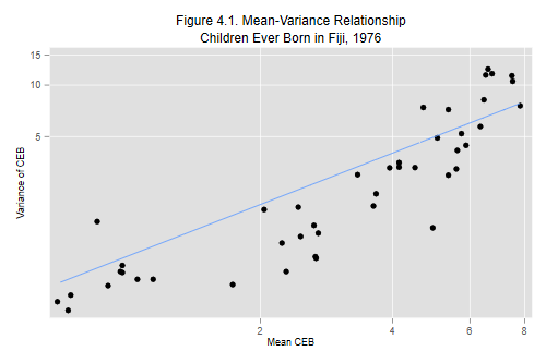
Clearly the variance increases with the mean. Most of the points lie below the 45 degree line, indicating that the variance is not exactly equal to the mean. Still, the assumption of proportionality brings us much closer to the data than the assumption of constant variance.
The dataset does not have information about the number of children ever born (CEB) to each woman, but it turns out that we can still model the mean by working with the cell totals and introducing the log of the number of women in the cell as an offset.
If the number of CEB to one woman in a given cell is a Poisson random variable with mean (and variance) μ, then the number born to all n women in that cell is a Poisson r.v. with mean (and variance) nμ. The log of the expected sum is log (n) + log (μ), and consists of a known offset plus the quantity we are interested in modeling. See the notes for further details
We therefore start by computing the outcome, the total CEB in each cell, and the offset.
. gen y = round( mean * n, 1)

. gen os = log(n)
We are ready to fit the null model, which has an offset but no predictors.
. poisson y, offset(os)

Iteration 0:   log likelihood =  -2080.664
Iteration 1:   log likelihood =  -2080.664

Poisson regression                                     Number of obs =      70
                                                       LR chi2(0)    =   -0.00
                                                       Prob > chi2   =       .
Log likelihood = -2080.664                             Pseudo R2     = -0.0000

─────────────┬────────────────────────────────────────────────────────────────
           y │ Coefficient  Std. err.      z    P>|z|     [95% conf. interval]
─────────────┼────────────────────────────────────────────────────────────────
       _cons │   1.376346   .0097119   141.72   0.000     1.357311    1.395381
          os │          1  (offset)
─────────────┴────────────────────────────────────────────────────────────────

. di exp(_b[_cons])
3.9604033

. quietly sum mean [fw=n]

. di r(mean)
3.9604968

. estat gof

         Deviance goodness-of-fit =  3731.851
         Prob > chi2(69)          =    0.0000

         Pearson goodness-of-fit  =  3375.349
         Prob > chi2(69)          =    0.0000
The constant is the log of the mean number of children ever born. Exponentiating we see that the estimated mean is almost four children per woman. The estimate coincides with the sample mean, as we verified by averaging the cell means with the number of women as a frequency weight.
The deviance of 3,732 on 69 d.f. gives a clear indication that the model doesn’t fit the data. The hypothesis that the expected number of CEB is the same for all women regardless of marriage duration, residence and education, is soundly rejected,
In rate models the offset usually represents the log of exposure, and
Stata lets us specify it directly using the offset() option
with the name of the variable representing the offset, or using the
exposure() option with the name of the variable
representing exposure, in which case Stata takes the log.
Next we fit the three one-factor models, starting with residence:
. poisson y i.res, offset(os)

Iteration 0:   log likelihood = -2051.3779
Iteration 1:   log likelihood = -2044.3868
Iteration 2:   log likelihood = -2044.3778
Iteration 3:   log likelihood = -2044.3778

Poisson regression                                      Number of obs =     70
                                                        LR chi2(2)    =  72.57
                                                        Prob > chi2   = 0.0000
Log likelihood = -2044.3778                             Pseudo R2     = 0.0174

─────────────┬────────────────────────────────────────────────────────────────
           y │ Coefficient  Std. err.      z    P>|z|     [95% conf. interval]
─────────────┼────────────────────────────────────────────────────────────────
         res │
      Urban  │   .1442896    .032448     4.45   0.000     .0806926    .2078866
      Rural  │   .2280596   .0278321     8.19   0.000     .1735097    .2826095
             │
       _cons │   1.204598   .0249922    48.20   0.000     1.155614    1.253581
          os │          1  (offset)
─────────────┴────────────────────────────────────────────────────────────────

. di exp(_b[2.res]), exp(_b[3.res])
1.1552186 1.2561602

. estat gof

         Deviance goodness-of-fit =  3659.279
         Prob > chi2(67)          =    0.0000

         Pearson goodness-of-fit  =  3304.611
         Prob > chi2(67)          =    0.0000
The estimates show that women in urban and rural areas have on average 16 and 26% more children than women in Suva. The model chi-squared of 73 on 2 d.f. tells us that this model is a significant improvement over the null. The deviance, still in the thousands, tells us that this model is far from fitting the data.
Now for education
. poisson y i.educ, offset(os)

Iteration 0:   log likelihood = -1588.3352
Iteration 1:   log likelihood = -1545.4751
Iteration 2:   log likelihood = -1545.2371
Iteration 3:   log likelihood = -1545.2371

Poisson regression                                     Number of obs =      70
                                                       LR chi2(3)    = 1070.85
                                                       Prob > chi2   =  0.0000
Log likelihood = -1545.2371                            Pseudo R2     =  0.2573

───────────────┬────────────────────────────────────────────────────────────────
             y │ Coefficient  Std. err.      z    P>|z|     [95% conf. interval]
───────────────┼────────────────────────────────────────────────────────────────
          educ │
Lower primary  │  -.2117869   .0216769    -9.77   0.000    -.2542729   -.1693008
Upper primary  │  -.6160532   .0288581   -21.35   0.000    -.6726141   -.5594922
   Secondary+  │  -1.224676   .0514108   -23.82   0.000     -1.32544   -1.123913
               │
         _cons │   1.647278   .0146932   112.11   0.000      1.61848    1.676076
            os │          1  (offset)
───────────────┴────────────────────────────────────────────────────────────────

. mata exp(st_matrix("e(b)"))
                 1             2             3             4             5
    ┌───────────────────────────────────────────────────────────────────────┐
  1 │            1   .8091371376   .5400718104   .2938527957   5.192824803  │
    └───────────────────────────────────────────────────────────────────────┘

. estat gof

         Deviance goodness-of-fit =  2660.997
         Prob > chi2(66)          =    0.0000

         Pearson goodness-of-fit  =  2426.918
         Prob > chi2(66)          =    0.0000
The estimates show that the number of CEB declines substantially with education. Women with secondary education or more have 71% fewer children than women with no education (or only 29% as many). The educational differential is highly significant, but this model doesn’t fit the data.
Finally, here’s duration:
. poisson y i.dur, offset(os)

Iteration 0:   log likelihood =  -315.2481
Iteration 1:   log likelihood = -297.80021
Iteration 2:   log likelihood = -297.77426
Iteration 3:   log likelihood = -297.77426

Poisson regression                                     Number of obs =      70
                                                       LR chi2(5)    = 3565.78
                                                       Prob > chi2   =  0.0000
Log likelihood = -297.77426                            Pseudo R2     =  0.8569

─────────────┬────────────────────────────────────────────────────────────────
           y │ Coefficient  Std. err.      z    P>|z|     [95% conf. interval]
─────────────┼────────────────────────────────────────────────────────────────
         dur │
        5-9  │   1.044886   .0523975    19.94   0.000     .9421893    1.147584
      10-14  │   1.444947   .0502397    28.76   0.000     1.346479    1.543416
      15-19  │   1.706756   .0497474    34.31   0.000     1.609253     1.80426
      20-24  │   1.877474   .0496492    37.81   0.000     1.780164    1.974785
        25+  │   2.078855    .047507    43.76   0.000     1.985743    2.171967
             │
       _cons │  -.1036046   .0441511    -2.35   0.019    -.1901391     -.01707
          os │          1  (offset)
─────────────┴────────────────────────────────────────────────────────────────

. estat gof

         Deviance goodness-of-fit =  166.0717
         Prob > chi2(64)          =    0.0000

         Pearson goodness-of-fit  =  156.3573
         Prob > chi2(64)          =    0.0000
Not surprisingly, the number of CEB is much higher for women who have been married longer. This is by far the most important predictor of CEB, with a chi-squared of 3,566 on just 5 d.f. In fact, a demographer wouldn’t even have looked at models that did not include a control for duration of marriage. It’s nice to see that Poisson regression can uncover the obvious :) Note that this model still doesn’t fit the data.
The deviances given in this section are pretty close to the deviances in Table 4.3 of the notes. You will notice small differences due to the use of different rounding procedures. In the notes we multiplied the mean CEB by the number of women and retained a few decimals. Here we rounded the total number of CEB to the nearest integer. If you omit the rounding you will reproduce the results in the notes exactly.
We now consider models that take two of the three factors into account. Following the notes we consider only models that include duration of marriage, an essential control when we study cumulative fertility. This leaves two models with main effects of two factors, and another two models that add one interaction.
Because we are only interested in deviances I will run the estimation commands quietly.
So here are the additive models
. quietly poisson y i.dur i.res , offset(os)

. quietly estat gof

. di "Deviance = ", r(chi2_d),"on", r(df),"d.f. p-value =",r(p_d)
Deviance =  120.68035 on 62 d.f. p-value = .00001189

. quietly poisson y i.dur i.educ, offset(os)

. quietly estat gof

. di "Deviance = ", r(chi2_d),"on", r(df),"d.f. p-value =",r(p_d)
Deviance =  100.19163 on 61 d.f. p-value = .00116423
And here are the models with one interaction
. quietly poisson y i.dur#i.res , offset(os)

. estat gof

         Deviance goodness-of-fit =  108.8965
         Prob > chi2(52)          =    0.0000

         Pearson goodness-of-fit  =  104.9353
         Prob > chi2(52)          =    0.0000

. quietly poisson y i.dur#i.educ, offset(os)

. estat gof

         Deviance goodness-of-fit =  84.53043
         Prob > chi2(46)          =    0.0005

         Pearson goodness-of-fit  =  84.69985
         Prob > chi2(46)          =    0.0004
The best fit so far is the model that includes duration and education, but it exhibits significant lack of fit with a chi-squared of 84.5 on 46 d.f.
We are now ready to look at models that include all three factors. We start with the additive model.
. poisson y i.dur i.res  i.educ, offset(os)

Iteration 0:   log likelihood = -623.59688
Iteration 1:   log likelihood = -252.64903
Iteration 2:   log likelihood = -250.07248
Iteration 3:   log likelihood = -250.07108
Iteration 4:   log likelihood = -250.07108

Poisson regression                                     Number of obs =      70
                                                       LR chi2(10)   = 3661.19
                                                       Prob > chi2   =  0.0000
Log likelihood = -250.07108                            Pseudo R2     =  0.8798

───────────────┬────────────────────────────────────────────────────────────────
             y │ Coefficient  Std. err.      z    P>|z|     [95% conf. interval]
───────────────┼────────────────────────────────────────────────────────────────
           dur │
          5-9  │   .9969348   .0527437    18.90   0.000     .8935591    1.100311
        10-14  │   1.369395   .0510688    26.81   0.000     1.269302    1.469488
        15-19  │   1.613757   .0511949    31.52   0.000     1.513417    1.714097
        20-24  │   1.784911   .0512138    34.85   0.000     1.684534    1.885288
          25+  │   1.976405   .0500341    39.50   0.000      1.87834     2.07447
               │
           res │
        Urban  │   .1124186   .0324963     3.46   0.001      .048727    .1761102
        Rural  │   .1516602   .0283292     5.35   0.000      .096136    .2071845
               │
          educ │
Lower primary  │   .0229728   .0226563     1.01   0.311    -.0214327    .0673783
Upper primary  │  -.1012738   .0309871    -3.27   0.001    -.1620073   -.0405402
   Secondary+  │  -.3101495   .0552107    -5.62   0.000    -.4183605   -.2019386
               │
         _cons │  -.1170972   .0549118    -2.13   0.033    -.2247222   -.0094721
            os │          1  (offset)
───────────────┴────────────────────────────────────────────────────────────────

. estat gof

         Deviance goodness-of-fit =   70.6653
         Prob > chi2(59)          =    0.1421

         Pearson goodness-of-fit  =  71.53348
         Prob > chi2(59)          =    0.1269
This model passes the goodness of fit hurdle, with a deviance of 70.67 on 59 d.f. and a corresponding P-value of 0.14, so we have no evidence against this model.
To exponentiate the parameter estimates we can reissue the
poisson command with the irr option, which is
short for incidence-rate ratios.
. poisson, irr

Poisson regression                                     Number of obs =      70
                                                       LR chi2(10)   = 3661.19
                                                       Prob > chi2   =  0.0000
Log likelihood = -250.07108                            Pseudo R2     =  0.8798

───────────────┬────────────────────────────────────────────────────────────────
             y │        IRR   Std. err.      z    P>|z|     [95% conf. interval]
───────────────┼────────────────────────────────────────────────────────────────
           dur │
          5-9  │   2.709963   .1429334    18.90   0.000     2.443812    3.005099
        10-14  │   3.932972   .2008521    26.81   0.000     3.558369     4.34701
        15-19  │   5.021644   .2570824    31.52   0.000     4.542226    5.551663
        20-24  │    5.95905   .3051855    34.85   0.000     5.389938    6.588254
          25+  │   7.216753   .3610835    39.50   0.000     6.542636    7.960327
               │
           res │
        Urban  │   1.118981   .0363628     3.46   0.001     1.049934    1.192569
        Rural  │   1.163765   .0329685     5.35   0.000     1.100909    1.230209
               │
          educ │
Lower primary  │   1.023239   .0231828     1.01   0.311     .9787954      1.0697
Upper primary  │   .9036856   .0280026    -3.27   0.001      .850435    .9602706
   Secondary+  │   .7333373    .040488    -5.62   0.000     .6581249    .8171451
               │
         _cons │   .8894988   .0488439    -2.13   0.033     .7987381    .9905726
            os │          1  (offset)
───────────────┴────────────────────────────────────────────────────────────────
Note: _cons estimates baseline incidence rate.
Briefly, the estimates indicate that the number of CEB increases rapidly with marital duration; in each category of residence and education women married 15-19 years have five times as many children as those married less than five years. Women who live in urban and rural areas have 12% and 16% more children than women who live in Suva and have the same marriage duration and education. Finally, more educated women have fewer children, as women with secondary or more education have on average 27% fewer children than women with no education who live in the same type of place of residence and have been married just as long.
We now put the additive model to some “stress tests” by considering
all possible interactions. The code below runs the models and
estat gof in a loop using quietly to save
space, printing just the model, deviance, d.f. and p-value for each
model.
. local heading "Model {col 37} Deviance {col 48} d.f. {col 57}p-value"

. foreach model in  "i.dur i.res##i.educ" "i.dur##i.res i.educ"  ///
>    "i.dur##i.educ i.res" "(i.dur i.res)##i.educ" "(i.dur i.educ)##i.res" ///
>    "i.dur##(i.res i.educ)" "i.dur##(i.res i.educ) i.res#i.educ" {
  2.     if "`heading'" != "" di "`heading'"
  3.     local heading = ""
  4.     quietly poisson y `model', offset(os)
  5.     quietly estat gof
  6.     di "`model'", _column(37) %8.2f r(chi2_d), ///
>       _column(47) %5.0f r(df), _column(57) %6.4f r(p_d)
  7. }
Model                                Deviance   d.f.    p-value
i.dur i.res##i.educ                    59.92     53     0.2391
i.dur##i.res i.educ                    57.13     49     0.1986
i.dur##i.educ i.res                    54.80     44     0.1274
(i.dur i.res)##i.educ                  44.52     38     0.2163
(i.dur i.educ)##i.res                  44.31     43     0.4162
i.dur##(i.res i.educ)                  42.65     34     0.1467
i.dur##(i.res i.educ) i.res#i.educ     30.86     28     0.3235
These calculations complete Table 4.3 in the notes. I reported the deviances for consistency with the notes, but could just as well have reported likelihood ratio tests comparing each of these models to the additive model. Make sure you know how to use the output to test, for example, whether we need to add a duration by education interaction. It should be clear from the list of deviances that we don’t need to add any of these terms. We conclude that the additive model does a fine job indeed.
It’s important to note that the need for interactions depends exactly on what’s being modeled. Here we used the log link, so all effects are relative. In this scale no interactions are needed. If we used the identity link we would be modeling the actual number of children ever born, and all effects would be absolute. In that scale we would need, at the very least, interactions with duration of marriage. See the notes for further discussion.
Updated fall 2022