
Two brief notes on the latent variable formulation of binary response models and the use of alternative links. First we plot three different links in a standardized scale. Second we compare logit and probit estimates for a model of contraceptive use.
Let us reproduce Figure 3.7, which shows the logit, probit and complementary log-log link, after standardizing the latent variable so it has mean 0 and variance 1. The probit link is based on the standard normal distribution, which is already standardized. The logit link is based on the standard logistic distribution, which has mean 0 and variance π2/3. The c-log-log link is based on the extreme value (log Weibull) distribution, with mean 0.577 and variance π2/6.
. twoway function y=normal(x), range(-2 2) lpat(solid) ///
>   || function y=invlogit(x*_pi/sqrt(3)), range(-2 2) lpat(dash) ///
>   || function y=1-exp(-exp(-0.577+x*_pi/sqrt(6))), range(-2 2) lpat(longdash) ///
>  , title("Figure 3.7: Probit, Logit and C-Log-Log Links") ///
>    subtitle(Standardized) ytitle(Probability) xtitle("Linear Predictor") ///
>    legend(order(1 "probit" 2 "logit" 3 "cloglog") cols(1) ring(0) pos(5))

. graph export fig37.png, width(500) replace
file fig37.png saved as PNG format
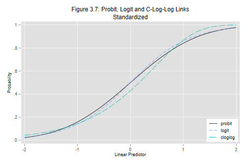
As you can see, the logit and probit links are virtually indistinguisable. The c-log-log link looks different, but one would still need very large sample sizes to be able to distinguish it from the others.
We will fit a probit model to the data on contraceptive use by age
and desire for more children. Following the notes we will pick the
specification where age is treated linearly and we include an
interaction between age and desire for no more children. To simplify
interpretation of the interaction we center age at 30 years. We use the
glm command to handle grouped data, see also
probit for individual data.
. //use https://grodri.github.io/datasets/cuse, clear
. use d:/dataweb/wws509/datasets/cusew, clear
(Contraceptive Use Data (Fiji, 1976))

. gen n = users + nonusers

. recode age (1=-10) (2=-2.5) (3=5) (4=15), gen(agemc)
(16 differences between age and agemc)

. glm users agemc nomore c.nomore#c.agemc, family(binomial n) link(probit)

Iteration 0:   log likelihood =  -50.26659
Iteration 1:   log likelihood = -50.256681
Iteration 2:   log likelihood = -50.256681

Generalized linear models                         Number of obs   =         16
Optimization     : ML                             Residual df     =         12
                                                  Scale parameter =          1
Deviance         =  29.00545504                   (1/df) Deviance =   2.417121
Pearson          =  28.31144084                   (1/df) Pearson  =   2.359287

Variance function: V(u) = u*(1-u/n)               [Binomial]
Link function    : g(u) = invnorm(u/n)            [Probit]

                                                  AIC             =   6.782085
Log likelihood   = -50.25668135                   BIC             =   -4.26561

─────────────────┬────────────────────────────────────────────────────────────────
                 │                 OIM
           users │ Coefficient  std. err.      z    P>|z|     [95% conf. interval]
─────────────────┼────────────────────────────────────────────────────────────────
           agemc │   .0128686   .0060884     2.11   0.035     .0009356    .0248017
          nomore │   .4389759   .0744411     5.90   0.000      .293074    .5848777
                 │
c.nomore#c.agemc │   .0304807   .0092269     3.30   0.001     .0123963    .0485651
                 │
           _cons │  -.7374078   .0453175   -16.27   0.000    -.8262284   -.6485872
─────────────────┴────────────────────────────────────────────────────────────────

. mat b_probit = e(b)'
Probit coefficients can be interpreted in terms of a standardized latent variable representing a propensity to use contraception, or the difference in expected utilities between using and not using contraception.
We see that the propensity among women who want more children increases with age at the rate of just over one tenth of a standard deviation per year. More interestingly, the propensity is 0.44 standard deviations higher among women who want no more children than among those who want more at age 30. This difference increases by 0.03 standard deviations per year of age, so it is 0.13 standard deviations at age 20 but 0.74 standard deviations at age 40. As a result, the propensity to use contraception among women who want no more children is 0.04 standard deviations higher per year of age.
It may be of interest to compare logit and probit coefficients. One way to compare them is to divide the logit coefficients by π/√3 = 1.8. This standardizes the logistic latent variable to have variance one, so the coefficients have the same interpretation as a probit model. The first two columns in the table below show that the two sets of coefficients are in fact very similar
. quietly glm users agemc nomore c.nomore#c.agemc, family(binomial n)

. mat b_logit = e(b)'

. mat both = b_probit, b_logit*sqrt(3)/_pi, b_logit/1.6

. mat colnames both = probit logit_std amemiya

. mat list both

both[4,3]
             probit   logit_std     amemiya
  users:
  agemc   .01286865   .01203162   .01363934
 nomore   .43897588   .40176118   .45544636
c.nomore#
c.agemc    .0304807   .02645902   .02999459
  _cons   -.7374078  -.66570995  -.75466517
Gelman and Hill (2007), following Amemiya (1981), recommend dividing by 1.6. This factor was chosen by trial and error to make the transformed logistic approximate the standard normal distribution over a wide domain. As shown in the third column above, it gives a somewhat closer approximation to the probit coefficients in our example, particularly for the interaction term. Of course the difference between dividing by 1.8 or 1.6 is not going to be large.
Gelman, A. and Hill, J. (2007) Data Analysis Using Regression and Multilevel/Hierarchical Models. Cambridge: Cambridge University Press.
Amemiya, T. (1981). Qualitative response models: a survey. Journal of Economic Literature, 19:1483–1536.
Updated fall 2022