
We now consider the comparison of more than two groups. We will illustrate using the data on contraceptive use by age, where we compare four groups.
These are the data on page 18 of the notes, entered as four age groups
. clear

. input ageg  users  nonusers

          ageg      users   nonusers
  1.   1  72 325
  2.   2 105 299
  3.   3 237 375
  4.   4  93 101
  5. end

. label define ageg 1 "<25" 2 "25-29" 3 "30-39" 4 "40-49"

. label values ageg ageg

. gen n = users + nonusers

. list

     ┌────────────────────────────────┐
     │  ageg   users   nonusers     n │
     ├────────────────────────────────┤
  1. │   <25      72        325   397 │
  2. │ 25-29     105        299   404 │
  3. │ 30-39     237        375   612 │
  4. │ 40-49      93        101   194 │
     └────────────────────────────────┘
Here is the model treating age as a factor with four levels, which is
of course saturated for the data. We will store the estimates for later
use. Stata can save estimates on disk using estimates save
or keep them in memory with estimates store. We’ll use the
latter.
. glm users i.ageg, family(binomial n)

Iteration 0:   log likelihood = -12.323383
Iteration 1:   log likelihood = -12.323383

Generalized linear models                         Number of obs   =          4
Optimization     : ML                             Residual df     =          0
                                                  Scale parameter =          1
Deviance         =  6.66091e-16                   (1/df) Deviance =          .
Pearson          =  4.31348e-20                   (1/df) Pearson  =          .

Variance function: V(u) = u*(1-u/n)               [Binomial]
Link function    : g(u) = ln(u/(n-u))             [Logit]

                                                  AIC             =   8.161692
Log likelihood   = -12.32338328                   BIC             =   6.66e-16

─────────────┬────────────────────────────────────────────────────────────────
             │                 OIM
       users │ Coefficient  std. err.      z    P>|z|     [95% conf. interval]
─────────────┼────────────────────────────────────────────────────────────────
        ageg │
      25-29  │   .4606758   .1727255     2.67   0.008     .1221401    .7992116
      30-39  │   1.048293   .1544406     6.79   0.000     .7455952    1.350991
      40-49  │   1.424638   .1939574     7.35   0.000     1.044488    1.804788
             │
       _cons │  -1.507159   .1302529   -11.57   0.000     -1.76245   -1.251868
─────────────┴────────────────────────────────────────────────────────────────

. estimates store mageg
Compare the parameter estimates with those on Table 3.5 of the notes.
Can you obtain these estimates by hand directly from the raw
frequencies? We see that the odds of using contraception increase
steadily from one age group to the next. You could type
glm, eform to convert from logit coefficients to odds
ratios.
To test the significance of the age effects we can use a likelihood
ratio test comparing this model with the null, or a Wald test. Let us
start with the former. In Stata we need to fit the null model, which we
do quietly, before using lrtest
. quietly glm users, family(binomial n)

. estimates store null

. estimates restore mageg // for later use
(results mageg are active now)

. lrtest null mageg

Likelihood-ratio test
Assumption: null nested within mageg

 LR chi2(3) =  79.19
Prob > chi2 = 0.0000
The value of 79.19 on 3 d.f. means that we can reject the hypothesis that the probability of using contraception is the same in the four age groups.
Now for the Wald test, which is easily obtained using the
testparm command. Here’s the test for the age effect on
page 20 of the notes:
. testparm i.ageg

 ( 1)  [users]2.ageg = 0
 ( 2)  [users]3.ageg = 0
 ( 3)  [users]4.ageg = 0

           chi2(  3) =   74.36
         Prob > chi2 =    0.0000
Once again the likelihood ratio and Wald test are similar, but not identical.
Finally, we will compute the fitted logits, which we will need later.
We can do this using the predict command, with the
xb option to make predictions in the scale of the linear
predictor, which in this case is the logit scale. (The default is to
predict in the scale of the response, in this case counts.)
. predict obslogit, xb
We will now treat age as a covariate, using the mid-points of the
four age groups; so we treat the group 15-24 as 20, 25-29 as 27.5, 30-39
as 35 and 40-49 as 45. (If these don’t look like mid-points to you, note
that age is usually reported in completed years, so 15-24 means between
15.0 and 25.0, and the mid-point is 20.0.) The easiest way to code the
midpoints in this example is via the recode command.
. recode ageg 1=20 2=27.5 3=35 4=45, gen(agem)
(4 differences between ageg and agem)
We can now fit the model on page 20 of the notes, which has a linear effect of age:
. glm users agem, family(binomial n)

Iteration 0:   log likelihood = -13.525129
Iteration 1:   log likelihood = -13.525059
Iteration 2:   log likelihood = -13.525059

Generalized linear models                         Number of obs   =          4
Optimization     : ML                             Residual df     =          2
                                                  Scale parameter =          1
Deviance         =  2.403351895                   (1/df) Deviance =   1.201676
Pearson          =  2.410763716                   (1/df) Pearson  =   1.205382

Variance function: V(u) = u*(1-u/n)               [Binomial]
Link function    : g(u) = ln(u/(n-u))             [Logit]

                                                  AIC             =    7.76253
Log likelihood   = -13.52505922                   BIC             =  -.3692368

─────────────┬────────────────────────────────────────────────────────────────
             │                 OIM
       users │ Coefficient  std. err.      z    P>|z|     [95% conf. interval]
─────────────┼────────────────────────────────────────────────────────────────
        agem │    .060671   .0071034     8.54   0.000     .0467486    .0745934
       _cons │  -2.672667   .2332492   -11.46   0.000    -3.129827   -2.215507
─────────────┴────────────────────────────────────────────────────────────────

. di exp(_b[agem])
1.0625493
We see that older women are more likely to use contraception, and that the odds of using contraception are about six percent higher for every year of age. (This comes from exponentiating the coefficient of age, which is now measured in years.)
We can formaly test the assumption of linearity using a likelihood
ratio test to compare this model with the saturated model of the
previous section. The test can be calculated using Stata’s
lrtest command, which uses a dot to refer to the
current model.
. lrtest . mageg

Likelihood-ratio test
Assumption: . nested within mageg

 LR chi2(2) =   2.40
Prob > chi2 = 0.3007
The chi-squared statistic of 2.4 on one d.f. is not significant, indicating that we have no evidence against the assumption of linearity, and can happily save two degrees of freedom. This statistic is, of course, the deviance for the model with a linear effect of age.
We can also calculate the deviance “by hand” from first principles, using the “sum of observed times log(observed/expected)” formula . Just remember that you need to use observed and expected counts of both successes and failures, here users and non-users:
. predict pusers // predicted count of users
(option mu assumed; predicted mean users)

. gen di = 2*(users*log(users/pusers) + (n-users)*log((n-users)/(n-pusers)))

. quietly summarize di

. display "Deviance = ", r(sum)
Deviance =  2.4033537
The next step will be to compute fitted logits based on this model, and use them together with the observed logits calculated earlier to examine visually the adequacy of the linear specification, effectively reproducing Figure 3.2 in the notes. For added measure I will also consider a model with a quadratic term, centering age around 30 before squaring it, so the linear term reflects the slope at 30.
. predict lfit1, xb

. gen agemcsq = (agem-30)^2

. quietly glm users agem agemcsq, family(binomial n)

. graph twoway (scatter obslogit agem) (line lfit1 agem) ///
>   (function f=_b[_cons]+_b[agem]*x+_b[agemcsq]*(x-30)^2, ///
>   range(20 45)) ///
>   ,   title("Figure 3.2: Observed and Fitted Logits By Age") ///
>       xtitle("age") ytitle("logit") legend(off)

. graph export fig32.png, width(500) replace
file fig32.png saved as PNG format
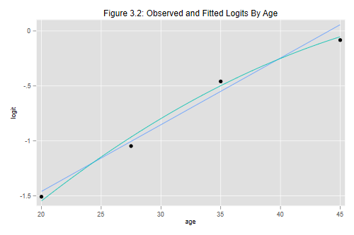
The graph shows that the linear specification was adequate. There is a hint that a quadratic model might be better, particularly in terms of the fit for the oldest age group, but the quadratic term is not significant.
You may wonder why I used functions to graph the fitted lines. Plotting the fitted values joined by line segments works fine for the linear model, but doesn’t reflect well the curvilinearity of the quadratic model, which is better represented using a function based on the coefficients.
This analysis gives us a quick indication of whether we could treat age linearly if we were working with individual data and had the actual ages of the 1607 women. It is not equivalent, however, because we have grouped age, and therefore treated all women men aged 25-29 as if they were age 27.5. With individual data some would be 25, some 26, etc.
You may also wonder why we were able to do a likelihood ratio test, when a model treating age linearly is usually not nested in a model that treats it as a factor. The answer is that in this case both specifications are applied to grouped data. You can view the linear model as imposing constraints, where the differences betwen the age groups are proportional to the difference in years between their midpoints. Alternatively, you can view the model that treats age as four groups as equivalent to having linear, quadratic, and cubic terms on the midpoints. Go ahead, try it. I’ll wait.
Updated fall 2022