A Poisson Model

Let us fit the model used by Long and Freese (2006), a simple additive model using all five predictors.

> mp <- glm(art~fem+mar+kid5+phd+ment, family=poisson, data=ab)
> summary(mp)

Call:
glm(formula = art ~ fem + mar + kid5 + phd + ment, family = poisson, 
    data = ab)

Deviance Residuals: 
    Min       1Q   Median       3Q      Max  
-3.5672  -1.5398  -0.3660   0.5722   5.4467  

Coefficients:
             Estimate Std. Error z value Pr(>|z|)    
(Intercept)  0.304617   0.102981   2.958   0.0031 ** 
fem         -0.224594   0.054613  -4.112 3.92e-05 ***
mar          0.155243   0.061374   2.529   0.0114 *  
kid5        -0.184883   0.040127  -4.607 4.08e-06 ***
phd          0.012823   0.026397   0.486   0.6271    
ment         0.025543   0.002006  12.733  < 2e-16 ***
---
Signif. codes:  0 '***' 0.001 '**' 0.01 '*' 0.05 '.' 0.1 ' ' 1

(Dispersion parameter for poisson family taken to be 1)

    Null deviance: 1817.4  on 914  degrees of freedom
Residual deviance: 1634.4  on 909  degrees of freedom
AIC: 3314.1

Number of Fisher Scoring iterations: 5

We see that the model obviously doesn’t fit the data. The five-percent critical value for a chi-squared with 909 d.f. is

> qchisq(0.95, df.residual(mp))

[1] 980.2518

> deviance(mp)

[1] 1634.371

> pr <- residuals(mp, "pearson")
> sum(pr^2)

[1] 1662.547

and the deviance and Pearson’s chi-squared are both in the 1600s.

Extra-Poisson Variation

We now assume that the variance is proportional rather than equal to the mean, and estimate the scale parameter \(\phi\) dividing Pearson’s chi-squared by its d.f.:

> phi <- sum(pr^2)/df.residual(mp)
> round(c(phi, sqrt(phi)), 4)

[1] 1.8290 1.3524

We see that the variance is about 83% larger than the mean. This means that we should adjust the standard errors multiplying by 1.35, the square root of 1.83.

R can do this calculation for us if we use the quasipoisson family:

> mq <- glm(art~fem+mar+kid5+phd+ment, family=quasipoisson, data=ab)
> summary(mq)

Call:
glm(formula = art ~ fem + mar + kid5 + phd + ment, family = quasipoisson, 
    data = ab)

Deviance Residuals: 
    Min       1Q   Median       3Q      Max  
-3.5672  -1.5398  -0.3660   0.5722   5.4467  

Coefficients:
             Estimate Std. Error t value Pr(>|t|)    
(Intercept)  0.304617   0.139273   2.187 0.028983 *  
fem         -0.224594   0.073860  -3.041 0.002427 ** 
mar          0.155243   0.083003   1.870 0.061759 .  
kid5        -0.184883   0.054268  -3.407 0.000686 ***
phd          0.012823   0.035700   0.359 0.719544    
ment         0.025543   0.002713   9.415  < 2e-16 ***
---
Signif. codes:  0 '***' 0.001 '**' 0.01 '*' 0.05 '.' 0.1 ' ' 1

(Dispersion parameter for quasipoisson family taken to be 1.829006)

    Null deviance: 1817.4  on 914  degrees of freedom
Residual deviance: 1634.4  on 909  degrees of freedom
AIC: NA

Number of Fisher Scoring iterations: 5

The estimates are exactly the same as before, but the standard errors are about 35% larger. We have essentially attributed all lack of fit to pure error. We can verify this fact easily. First we write a useful function to extract standard errors and then use it on our fits:

> se <- function(model) sqrt(diag(vcov(model)))
> round(data.frame(p=coef(mp), q=coef(mq), 
+   se.p=se(mp), se.q=se(mq), ratio=se(mq)/se(mp)), 4)

                  p       q   se.p   se.q  ratio
(Intercept)  0.3046  0.3046 0.1030 0.1393 1.3524
fem         -0.2246 -0.2246 0.0546 0.0739 1.3524
mar          0.1552  0.1552 0.0614 0.0830 1.3524
kid5        -0.1849 -0.1849 0.0401 0.0543 1.3524
phd          0.0128  0.0128 0.0264 0.0357 1.3524
ment         0.0255  0.0255 0.0020 0.0027 1.3524

An alternative approach is to fit a Poisson model and use the robust or sandwich estimator of the standard errors. This usually gives results very similar to the over-dispersed Poisson model.

Negative Binomial Regression

We now fit a negative binomial model with the same predictors. To do this we need the glm.nb() function in the MASS package.

> library(MASS)
> mnb <- glm.nb(art ~ fem + mar + kid5 + phd + ment, data = ab)   
> summary(mnb)

Call:
glm.nb(formula = art ~ fem + mar + kid5 + phd + ment, data = ab, 
    init.theta = 2.264387695, link = log)

Deviance Residuals: 
    Min       1Q   Median       3Q      Max  
-2.1678  -1.3617  -0.2806   0.4476   3.4524  

Coefficients:
             Estimate Std. Error z value Pr(>|z|)    
(Intercept)  0.256144   0.137348   1.865 0.062191 .  
fem         -0.216418   0.072636  -2.979 0.002887 ** 
mar          0.150489   0.082097   1.833 0.066791 .  
kid5        -0.176415   0.052813  -3.340 0.000837 ***
phd          0.015271   0.035873   0.426 0.670326    
ment         0.029082   0.003214   9.048  < 2e-16 ***
---
Signif. codes:  0 '***' 0.001 '**' 0.01 '*' 0.05 '.' 0.1 ' ' 1

(Dispersion parameter for Negative Binomial(2.2644) family taken to be 1)

    Null deviance: 1109.0  on 914  degrees of freedom
Residual deviance: 1004.3  on 909  degrees of freedom
AIC: 3135.9

Number of Fisher Scoring iterations: 1

              Theta:  2.264 
          Std. Err.:  0.271 

 2 x log-likelihood:  -3121.917 

> 1/mnb$theta

[1] 0.4416205

> -2*(logLik(mp) - logLik(mnb))

'log Lik.' 180.196 (df=6)

R’s theta is the precision of the multiplicative random effect, and corresponds to \(1/\sigma^2\) in the notes. The estimate corresponds to an estimated variance of 0.44 and is highly significant.

To test the significance of this parameter you may think of computing twice the difference in log-likelihoods between this model and the Poisson model, 180.2, and treating it as a chi-squared with one d.f. The usual asymptotics do not apply, however, because the null hypothesis is on a boundary of the parameter space.

There is some work showing that a better approximation is to treat the statistic as as 50:50 mixture of zero and a chi-squared with one d.f. Alternatively, treating the statistic as a chi-squared with one d.f. gives a conservative test. Either way, we have overwhelming evidence of overdispersion.

For testing hypotheses about the regression coefficients we can use either Wald tests or likelihood ratio tests, which are possible because we have made full distributional assumptions.

There’s also a negative.binomial family for glm and this can be used provided the parameter theta is given. (This is based on the result that the negative binomial is in the glm family for fixed variance.) Here’s a quick check:

> mnbg <- glm(art~fem+mar+kid5+phd+ment, 
+   family=negative.binomial(mnb$theta), data=ab)
> all(abs(coef(mnb)-coef(mnbg)) < 1e-5)

[1] TRUE

The standard errors would differ, however, because glm.nb allows for the fact that theta was estimated, whereas glm does not.

Unobserved Heterogeneity

Let us draw the density of the parameter representing unobserved heterogeneity. R has a function dgamma(x, shape, rate = 1, scale = 1/rate) to compute the density of a gamma distribution with given shape and scale (or its reciprocal the rate). In particular, when the random effect has variance v the density is dgamma(x, shape = 1/v, scale = v).

> library(ggplot2)
> v = 1/mnb$theta
> x  = seq(0, 3, 0.05)
> gd = data.frame(x, g = dgamma(x, shape = 1/v, scale = v))
> png("gamdenr.png", width=500, height=400)
> ggplot(gd, aes(x, g)) + geom_line() + 
+ ggtitle("The Gamma Density for Heterogeneity with Variance 0.44")
> dev.off()

svg 
  2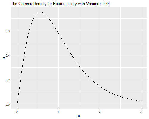 

We can also compute quantiles using qgamma(p, shape, rate = 1, scale = 1/rate, lower.tail = TRUE). In our case the shape is 1/v and the scale is v.

> qgamma((1:3)/4, shape = 1/v, scale = v)

[1] 0.5114167 0.8572697 1.3347651

Biochemists at Q1 of the distribution of unobserved heterogeneity publish 49% fewer papers than expected from their observed characteristics, while those at the median publish 14% fewer and those at Q3 publish 33% more than expected.

Comparing Estimates and Standard Errors

Let us compare parameter estimates and standard errors under the Poisson, over-dispersed Poisson and negative binomial models:

> round(data.frame(
+   p=coef(mp),q=coef(mq),nb=coef(mnb),
+ se.p=se(mp),se.q=se(mq),se.nb=se(mnb)),4)

                  p       q      nb   se.p   se.q  se.nb
(Intercept)  0.3046  0.3046  0.2561 0.1030 0.1393 0.1373
fem         -0.2246 -0.2246 -0.2164 0.0546 0.0739 0.0726
mar          0.1552  0.1552  0.1505 0.0614 0.0830 0.0821
kid5        -0.1849 -0.1849 -0.1764 0.0401 0.0543 0.0528
phd          0.0128  0.0128  0.0153 0.0264 0.0357 0.0359
ment         0.0255  0.0255  0.0291 0.0020 0.0027 0.0032

The negative binomial estimates are not very different from those based on the Poisson model, and both sets would led to the same conclusions.

Looking at the standard errors, we see that both approaches to over-dispersion lead to very similar estimated standard errors, and that ordinary Poisson regression underestimates the standard errors.

Goodness of Fit

We can assess the goodness of fit of the negative binomial model by using the deviance.

> deviance(mnbg)

[1] 1004.281

The negative binomial model fits better than the Poisson, but still has a deviance above the five percent critical value of 980.25.

The Variance Function

The over-dispersed Poisson and negative binomial models have different variance functions. One way to check which one may be more appropriate is to create groups based on the linear predictor, compute the mean and variance for each group, and finally plot the mean-variance relationship.

Here are groups based on the negative binomial linear predictor, created using cut() with breaks at the (5(5)95 percentiles to produce twenty groups of approximately equal size. Note that predict() computes a linear predictor, unless otherwise specified. To predict in the scale of the response add the option type="response".

> library(dplyr)

Attaching package: 'dplyr'

The following object is masked from 'package:MASS':

    select

The following objects are masked from 'package:stats':

    filter, lag

The following objects are masked from 'package:base':

    intersect, setdiff, setequal, union

> xb <- predict(mnb)
> q <- c(min(xb)-0.1, quantile(xb, seq(5,95,5)/100), max(xb)+0.1)
> ab <- mutate(ab, group=cut(xb, breaks=q))
> mv <- group_by(ab,group) |> summarize(mean=mean(art), variance=var(art), n=n())
> x <- seq(0.63, 3.37, 0.02)
> g  <- data.frame( mean = x, poisson = x * phi, negbin = x * (1 + x/mnb$theta))
> png("c4afig1r.png", width=500, height=400)
> ggplot(mv, aes(x=mean, y=variance)) + geom_point()  + xlim(0.5, 3.8) + 
+   geom_line(data=g, aes(x=mean, y=poisson) , linetype="dashed") +
+   geom_line(data=g, aes(x=mean, y=negbin), linetype="solid") +
+   ggtitle("Mean-Variance Relationship", 
+     subtitle = "Articles Published by Ph.D. biochemists") +
+   geom_text(x=3.6, y=6.2, label="P") + geom_text(x=3.6, y=8.5, label="NB") 
> dev.off()

svg 
  2 

The graph plots the mean versus the variance and overlays the curves corresponding to the over-dispersed Poisson model, where the variance is \(\phi\mu\), and the negative binomial model, where the variance is \(\mu(1+\mu\sigma^2)\).

The Poisson variance function does a pretty good job for the bulk of the data, but fails to capture the high variances of the most productive scholars. The negative binomial variance function is not too different but, being a quadratic, can rise faster and does a better job at the high end. We conclude that the negative binomial model provides a better description of the data than the over-dispersed Poisson model.

Zero-Inflated Poisson Models

A frequent occurrence with count data is an excess of zeroes compared to what’s expected under a Poisson model. This is actually a problem with our data:

> zobs <- ab$art == 0
> zpoi <- exp(-exp(predict(mp))) # or dpois(0,exp(predict(mp)))
> c(obs=mean(zobs), poi=mean(zpoi))

      obs       poi 
0.3005464 0.2092071 

We see that 30.0% of the scientists in the sample published no articles in the last three years of their Ph.D., but the Poisson model predicts that only 20.9% would have no publications. Clearly the model underestimates the probability of zero counts.

One way to model this type of situation is to assume that the data come from a mixture of two populations, one where the counts is always zero, and another where the count has a Poisson distribution with mean \(\mu\). In this model zero counts can come from either population, while positive counts come only from the second one.

In the context of publications by Ph.D. biochemists, we can imagine that some had in mind jobs where publications wouldn’t be important, while others were aiming for academic jobs where a record of publications was expected. Members of the first group would publish zero articles, whereas members of the second group would publish 0,1,2,…, a count that may be assumed to have a Poisson distribution.

The distribution of the outcome can then be modeled in terms of two parameters, \(\pi\) the probability of “always zero”, and \(\mu\), the mean number of publications for those not in the “always zero” group. A natural way to introduce covariates is to model the logit of the probability \(\pi\) of always zero and the log of the mean \(\mu\) for those not in the always zero class.

This type of model can be fit in R using the zeroinfl() function in the pscl package. The model formula can be specified as usual if the same variables are to be included in both equations. Otherwise one can provide two sets of predictors separated by a vertical bar, type ?zeroinfl to learn more.

Here’s a zero-inflated model with all covariates in both equations:

> library(pscl)

Classes and Methods for R developed in the
Political Science Computational Laboratory
Department of Political Science
Stanford University
Simon Jackman
hurdle and zeroinfl functions by Achim Zeileis

> mzip <- zeroinfl(art ~ fem + mar + kid5 + phd + ment, data=ab)
> summary(mzip)

Call:
zeroinfl(formula = art ~ fem + mar + kid5 + phd + ment, data = ab)

Pearson residuals:
    Min      1Q  Median      3Q     Max 
-2.3253 -0.8652 -0.2826  0.5404  7.2976 

Count model coefficients (poisson with log link):
             Estimate Std. Error z value Pr(>|z|)    
(Intercept)  0.640839   0.121307   5.283 1.27e-07 ***
fem         -0.209144   0.063405  -3.299 0.000972 ***
mar          0.103750   0.071111   1.459 0.144567    
kid5        -0.143320   0.047429  -3.022 0.002513 ** 
phd         -0.006166   0.031008  -0.199 0.842376    
ment         0.018098   0.002294   7.888 3.07e-15 ***

Zero-inflation model coefficients (binomial with logit link):
             Estimate Std. Error z value Pr(>|z|)   
(Intercept) -0.577060   0.509386  -1.133  0.25728   
fem          0.109752   0.280082   0.392  0.69517   
mar         -0.354018   0.317611  -1.115  0.26501   
kid5         0.217095   0.196483   1.105  0.26920   
phd          0.001275   0.145263   0.009  0.99300   
ment        -0.134114   0.045243  -2.964  0.00303 **
---
Signif. codes:  0 '***' 0.001 '**' 0.01 '*' 0.05 '.' 0.1 ' ' 1 

Number of iterations in BFGS optimization: 19 
Log-likelihood: -1605 on 12 Df

Looking at the inflate equation we see that the only significant predictor of being in the “always zero” class is the number of articles published by the mentor, with each article by the mentor associated with 12.6% lower odds of never publishing.

Looking at the equation for the mean number or articles among those not in the always zero class, we find significant disadvantages for females and scientists with children under five, and a large positive effect of the number of publications by the mentor, with each article associated with a 1.8% increase in the expected number of publications.

To verify that the model solves the problem of excess zeroes we predict \(\pi\) and \(\mu\), and calculate the combined probability of no publications. There are options in the predict() function called "zero" and "count" to obtain these. There’s also an option "prob" to compute the predicted density, but this is overkill, as we only want the probability of zero.

> pr <- predict(mzip,type="zero")  # pi
> mu <- predict(mzip,type="count") # mu
> zip <- pr + (1-pr)*exp(-mu)      # or predict(mzip,type="prob")[,1]
> mean(zip)

[1] 0.2985679

So the model solves the problem of excess zeroes, predicting that 29.9% of the biochemists will publish no articles, extremely close to the observed value of 30.0%.

There’s also a zero-inflated negative binomial model, which uses a negative binomial for the count in the “not always zero” class. This model can be fit using zeroinfl() with the dist="negbin" parameter. Alternative links for the inflate equation include the probit, which can be specified using link="probit".

Model Comparison with AIC

As it happens, for this data the negative binomial solves the problem of zeroes too! Here’s the probability of zero articles in the negative binomial. We proceed from first principles, but one could also use the built-in negative binomial density

> munb <- exp(predict(mnb))
> theta <- mnb$theta
> znb <- (theta/(munb+theta))^theta
> # also dnbinom(0, mu=munb, size=theta)
> mean(znb)

[1] 0.3035957

The model predicts that 30.4% of the biochemists would publish no articles in the last three years of their Ph.D., very close to the observed value of 30.0%.

To choose between the negative binomial and zero inflated models we need to resort to other criteria. A very simple way to compare models with different numbers of parameters is to compute Akaike’s Information Criterion (AIC), which we define as

AIC = -2logL + 2p

where p is the number of parameters in the model. The first term is essentially the deviance and the second a penalty for the number of parameters. I will obtain it “by hand” so we see exactly what’s going on. AIC may also be calculated using the AIC() function.

> c(nb = AIC(mnb), zip = AIC(mzip))

      nb      zip 
3135.917 3233.546 

> mzip$rank <- length(coef(mzip)) # add a rank component
> aic <- function(model) -2*logLik(model) + 2*model$rank
> sapply(list(mnb, mzip), aic)

[1] 3133.917 3233.546

For this dataset the negative binomial model is a clear winner in terms of parsimony and goodness of fit.

Additional diagnostic criteria we could look at are the marginal distribution of predicted and observed counts, and the variance functions.

References

Long, J.S. (1990). The Origins of Sex Differences in Science. Social Forces, 68:1297-1315.

Long, J.S. and Freese, J. (2006) Regression Models for Categorical Dependent Variables Using Stata. Second Edition. College Station, Texas: Stata Press.

Zeileis, A, Kleiber, C and Jackman, S. (2008). Regression Models for Count Data in R. Journal of Statistical Software, 27(8):1-25. URL https://www.jstatsoft.org/article/view/v027i08.

Updated fall 2022