Housing Conditions in Copenhagen

We will use data from 1681 residents of twelve areas in Copenhagen, classified in terms of the type of housing that they have (tower blocks, apartments, atrium houses and terraced houses), their feeling of influence on apartment management (low, medium, high), their degree of contact with the neighbors (low, high), and their satisfaction with housing conditions (low, medium, high).

The data are available in the datasets section and can be read directly from there.

> copen <- read.table("https://grodri.github.io/datasets/copen.dat")
> head(copen)

  housing influence contact satisfaction  n
1   tower       low     low          low 21
2   tower       low     low       medium 21
3   tower       low     low         high 28
4   tower       low    high          low 14
5   tower       low    high       medium 19
6   tower       low    high         high 37

We will treat satisfaction as the outcome and type of housing, feeling of influence and contact with the neighbors as categorical predictors. The data are grouped as in the earlier example, but the layout is long rather than wide. It corresponds to the way one would enter individual data, with an additional colum n showing the number of observations in each group.

It will be useful for comparison purposes to fit the saturated multinomial logit model, where each of the 24 combinations of housing type, influence and contact, has its own multinomial distribution. The group code can easily be generated from the observation number, and the easiest way to fit the model is to treat the code as a factor.

> copen$group <- rep(1:24,rep(3,24))
> library(nnet)
> msat <- multinom(satisfaction~as.factor(group), weights=n, data=copen)

# weights:  75 (48 variable)
initial  value 1846.767257 
iter  10 value 1723.705246
iter  20 value 1716.225889
iter  30 value 1715.715730
final  value 1715.710848 
converged

> logLik(msat)

'log Lik.' -1715.711 (df=48)

The log likelihood is -1715.7. You can verify that this is sum(n*log(p)), where n are the counts and p the proportions for the categories of satisfaction within each of the 24 groups.

The Proportional Odds Model

The next task is to fit the additive ordered logit model from Table 6.5 in the notes. I will use the polr() function in Venables and Rilpey’s MASS package. Before fitting, I relevel the predictors so the reference cells are tower residents, low influence, and low contact. I also make sure the outcome categories are ordered from low to high satisfaction.

> library(MASS)

Warning: package 'MASS' was built under R version 4.2.2

> library(dplyr)    

Attaching package: 'dplyr'

The following object is masked from 'package:MASS':

    select

The following objects are masked from 'package:stats':

    filter, lag

The following objects are masked from 'package:base':

    intersect, setdiff, setequal, union

> copen <- mutate(copen,  
+   satisfaction = ordered(satisfaction, levels=c("low","medium","high")),
+   housing = relevel(as.factor(housing), "tower"),
+   influence = relevel(as.factor(influence),"low"),
+   contact = relevel(as.factor(contact),"low"))
> madd <- polr(satisfaction ~ housing + influence + contact, 
+   weights=n, data=copen)
> summary(madd)

Re-fitting to get Hessian

Call:
polr(formula = satisfaction ~ housing + influence + contact, 
    data = copen, weights = n)

Coefficients:
                    Value Std. Error t value
housingapartments -0.5724    0.11924  -4.800
housingatrium     -0.3662    0.15517  -2.360
housingterraced   -1.0910    0.15149  -7.202
influencehigh      1.2888    0.12716  10.136
influencemedium    0.5664    0.10465   5.412
contacthigh        0.3603    0.09554   3.771

Intercepts:
            Value   Std. Error t value
low|medium  -0.4961  0.1248    -3.9739
medium|high  0.6907  0.1255     5.5049

Residual Deviance: 3479.149 
AIC: 3495.149 

> logLik(madd)

'log Lik.' -1739.575 (df=8)

> lrtest <- function(small, large) {
+    data.frame(chisq=deviance(small)-deviance(large), df=large$edf-small$edf)
+ }
> lrtest(madd, msat)

    chisq df
1 47.7276 40

The log-likelihood is -1739.6, so the deviance for this model compared to the saturated multinomial model is 47.7 on 40 d.f. polr() calculates the deviance of this model as -2logL, efectively comparing it to a saturated individual model. I prefer to compare with a multinomial model which is saturated for the 24 groups, which is why I calculate a difference in deviances, the same as twice a difference in log likelihoods.

The bottom line is that the deviance is not much more than one would expect when saving 40 parameters, so we have no evidence against the additive model. To be thorough, however, we will explore individual interactions just in case the deviance is concentrated on a few d.f.

Models with Interactions

The next step is to explore two-factor interactions.

> mhi <- polr(satisfaction ~ housing*influence + contact, weights=n, data=copen)
> lrtest(mhi, msat)

     chisq df
1 25.21826 34

> mhc <- polr(satisfaction ~ housing*contact + influence, weights=n, data=copen)
> lrtest(mhc, msat)

     chisq df
1 39.06145 37

> mic <- polr(satisfaction ~ housing + influence*contact, weights=n, data=copen)
> lrtest(mic, msat)

     chisq df
1 47.51865 38

The interaction between housing and influence reduces the deviance by about half, at the expense of only six d.f., so it is worth a second look. The interaction between housing and contact makes a much smaller dent, and the interaction between influence and contact adds practically nothing.

We could also compare each of these models to the additive model, thus testing the interaction directly. We would get chisquareds of 22.51 on 6 d.f., 8.67 on 3 d.f. and 0.21 on 2 d.f. You can obtain these using our handy lrtest() function, try for example lrtest(madd, mhi), which we’ll use below.

Clearly the interaction to add is the first one, allowing the association between satisfaction with housing and a feeling of influence on management, net of contact with neighbors, to depend on the type of housing. To examine parameter estimates we refit the model:

> summary(mhi)

Re-fitting to get Hessian

Call:
polr(formula = satisfaction ~ housing * influence + contact, 
    data = copen, weights = n)

Coefficients:
                                    Value Std. Error t value
housingapartments                 -1.1885    0.19724 -6.0256
housingatrium                     -0.6067    0.24457 -2.4808
housingterraced                   -1.6062    0.24100 -6.6650
influencehigh                      0.8689    0.27434  3.1671
influencemedium                   -0.1390    0.21255 -0.6541
contacthigh                        0.3721    0.09599  3.8764
housingapartments:influencehigh    0.7198    0.32873  2.1896
housingatrium:influencehigh       -0.1555    0.41048 -0.3789
housingterraced:influencehigh      0.8446    0.43027  1.9630
housingapartments:influencemedium  1.0809    0.26585  4.0657
housingatrium:influencemedium      0.6511    0.34500  1.8873
housingterraced:influencemedium    0.8210    0.33067  2.4829

Intercepts:
            Value   Std. Error t value
low|medium  -0.8882  0.1672    -5.3135
medium|high  0.3126  0.1657     1.8871

Residual Deviance: 3456.64 
AIC: 3484.64 

> lrtest(mhi, msat)

     chisq df
1 25.21826 34

> lrtest(madd, mhi)

     chisq df
1 22.50935  6

The model deviance of 25.2 on 34 d.f. is not significant. To test for the interaction effect we compare this model with the additive model, obtaining a chi-squared statistic of 22.5 on six d.f., which is significant at the 0.001 level.

At this point one might consider adding a second interaction. The obvious choice is to allow the association between satisfaction and contact with neighbors to depend on the type of housing. This would reduce the deviance by 7.95 at the expense of three d.f., a gain that just makes the conventional 5% cutoff with a p-value of 0.047. In the interest of simplicity, however, we will not pursue this addition.

Interpretation of Parameter Estimates

The estimates indicate that respondents who have high contact with their neighbors are more satisfied than respondents with low contact who live in the same type of housing and have the same feeling of influence on management. The difference is estimated as 0.372 units in the underlying logistic scale. Dividing by the standard deviation of the (standard) logistic distribution we obtain

> coef(mhi)["contacthigh"]/(pi/sqrt(3))

contacthigh 
  0.2051395 

So the difference in satisfaction between high and low contact with neighbors, among respondents with the same housing and influence, is 0.205 standard deviations.

Alternatively, we can exponentiate the coefficient:

> exp(coef(mhi)["contacthigh"])

contacthigh 
   1.450752 

The odds of reporting high satisfaction (relative to medium or low), are 45% higher among tenants who have high contact with the neighbors than among tenants with low contact and have the same type of housing and influence. The odds of reporting medium or high satisfaction (as opposed to low) are also 45% higher in this comparison.

Interpretation of the effects of housing type and influence requires taking into account the interaction effect. In the notes we describe differences by housing type among those who feel they have little influence in management, and the effects of influence in each type of housing.

Let us do something a bit different here, and focus on the joint effects of housing and influence, combining the main effects and interactions. To do this I extract the linear predictor for each combination of housing and influence, and create a matrix suitable for a bar plot. I also divide the estimates by π/√3 to express them in standard deviation units in a latent satisfaction scale.

> xb <- model.matrix(mhi) %*% c(0,coef(mhi))
> indices<-(1:nrow(copen))[copen$satisfaction=="low" & copen$contact=="low"]
> XB <- matrix(xb[indices],3,4)
> colnames(XB) <- levels(copen$housing)
> rownames(XB) <- levels(copen$influence)
> trio <- c("#ddeeff","#80aae6", "#3366cc")
> png("fig63r.png", width=500, height=400)
> barplot(XB, beside=TRUE, col=trio, border=NA, 
+   main="Joint Effects of Housing and Influence", col.main="#3366cc")
>  dev.off()

png 
  2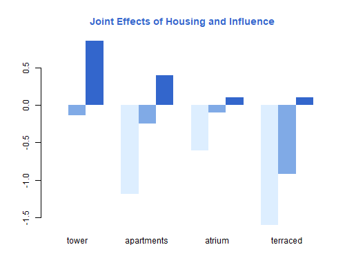 

Satisfaction with housing conditions is highest for residents of tower blocks who feel they have high influence, and lowest for residents of terraced houses with low influence. Satisfaction increases with influence in each type of housing, but the difference is largest for terraced houses and apartments than fower blocks and atrium houses.

Another way to present the results is by focusing on the effects of influence within each type of housing or, alternatively, on the effects of housing type within each category of influence. All we need to do is substract the values for the reference cell of the control variable. These, of course, are in the first row or column of our matrix,

> quartet  <- c("#ddeeff", "#9dc1ee","#6593dd", "#3366cc")
> png("fig64r.png", width=750, height=400)
> par(mfrow=c(1,2))
> barplot(apply(XB,2,function(x)x-x[1]), beside=TRUE, col=trio, 
+   border=NA, main="Effects of Influence Given Housing", col.main="#3366cc")
> legend("toplef", fill=trio, legend=levels(copen$influence), bty="n")
> barplot(apply(XB, 1, function(x)x-x[1]), beside=TRUE, col=quartet, 
+   border=NA, main="Effects of Housing Given Influence", col.main="#3366cc")
> legend("bottomright", fill=quartet, legend=levels(copen$housing), bty="n")
> dev.off()

png 
  2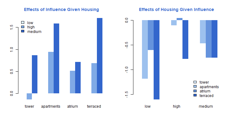 

On the left panel we see more clearly the differences by influence in each type of housing. As noted above, having influence is good, particularly of you live in a terraced house or apartment. The right panel shows differences by type of housing within categories of influence. Tower residents are, generally speaking, more satisfied than residents of other types of housing, and the differences tend to be larger when influence is low.

Estimation of Probabilities

Let us consider predicted probabilities. The predict() method can predict the outcome, with type="class" (the default), or the probabilities, with type="p". We’ll use the latter.

> copen <- mutate(copen, fitted=predict(mhi, type="p"))

We’ll look at these results for tower block dwellers with little influence and with high and low contact with neighbors. The first of these groups is, of course, the reference cell. I add the condition ‘satisfaction==“low”’ to list the probabilities just once for each group:

> filter(copen, housing=="tower" & influence=="low" & satisfaction=="low") |>
+     select(housing, influence, contact, fitted)

  housing influence contact fitted.low fitted.medium fitted.high
1   tower       low     low  0.2914869     0.2860400   0.4224731
4   tower       low    high  0.2209299     0.2642112   0.5148588

We see that among tower tenants with low influence, those with high contact with their neighbors have a higher probability of high satisfaction and a lower probability of medium or low satisfaction, than those with low contact with the neighbors.

It is instructive to reproduce these calculations “by hand”. For the reference cell all we need are the cutpoints. Remember that the model predicts cumulative probabilities, which is why we difference the results. We write a helper function to facilitate converting cumulative logits to probabilities. The cutpoints or intercepts are stored in a slot named zeta.

> xb2p <- function(xb, cdf=plogis) { 
+   p <- cdf(as.numeric(xb))
+   data.frame(low=p[1], medium=p[2]-p[1], high=1-p[2])
+ }
> xb2p(mhi$zeta)

        low  medium      high
1 0.2914869 0.28604 0.4224731

For the group with high contact we need to subtract the corresponding coefficient from the cutpoints. The change of sign is needed to convert coefficients from the latent variable to the cumulative probability formulations (or from upper to lower tails).

> xb2p(mhi$zeta - coef(mhi)["contacthigh"])

        low    medium      high
1 0.2209299 0.2642112 0.5148588

Results agree exactly with the earlier predicted probabilities.

The Ordered Probit Model

We now consider ordered probit models, starting with the additive model in Table 6.6:

> mpadd <- polr(satisfaction  ~ housing + influence + contact, weights=n,
+   method="probit", data=copen)
> summary(mpadd)

Re-fitting to get Hessian

Call:
polr(formula = satisfaction ~ housing + influence + contact, 
    data = copen, weights = n, method = "probit")

Coefficients:
                    Value Std. Error t value
housingapartments -0.3475    0.07229  -4.807
housingatrium     -0.2179    0.09477  -2.299
housingterraced   -0.6642    0.09180  -7.235
influencehigh      0.7829    0.07643  10.244
influencemedium    0.3464    0.06414   5.401
contacthigh        0.2224    0.05812   3.826

Intercepts:
            Value   Std. Error t value
low|medium  -0.2998  0.0762    -3.9371
medium|high  0.4267  0.0764     5.5850

Residual Deviance: 3479.689 
AIC: 3495.689 

> logLik(mpadd)

'log Lik.' -1739.844 (df=8)

> deviance(mpadd) - deviance(msat)

[1] 48.26715

The model has a log-likelihood of -1739.8, a little bit below that of the additive ordered logit. This is also reflected in the slightly higher deviance.

Next we add the housing by influence interaction

> mphi <- polr(satisfaction  ~ housing * influence + contact, weights=n,
+   method="probit", data=copen)
>  summary(mphi)

Re-fitting to get Hessian

Call:
polr(formula = satisfaction ~ housing * influence + contact, 
    data = copen, weights = n, method = "probit")

Coefficients:
                                     Value Std. Error t value
housingapartments                 -0.72806    0.12050 -6.0419
housingatrium                     -0.37207    0.15103 -2.4636
housingterraced                   -0.97900    0.14559 -6.7245
influencehigh                      0.51646    0.16393  3.1504
influencemedium                   -0.08637    0.13033 -0.6627
contacthigh                        0.22846    0.05832  3.9176
housingapartments:influencehigh    0.44791    0.19707  2.2729
housingatrium:influencehigh       -0.07797    0.24965 -0.3123
housingterraced:influencehigh      0.52167    0.25873  2.0163
housingapartments:influencemedium  0.66001    0.16258  4.0596
housingatrium:influencemedium      0.41084    0.21338  1.9254
housingterraced:influencemedium    0.49638    0.20164  2.4617

Intercepts:
            Value   Std. Error t value
low|medium  -0.5440  0.1023    -5.3150
medium|high  0.1892  0.1018     1.8574

Residual Deviance: 3457.331 
AIC: 3485.331 

> logLik(mphi)

'log Lik.' -1728.665 (df=14)

> deviance(mphi) - deviance(msat)

[1] 25.90907

> coef(mphi)["contacthigh"]

contacthigh 
  0.2284566 

We now have a log-likelihood of -1728.7 and a deviance of 25.9. which is almost indistinguishable from the corresponding ordered logit model.

The estimates indicate that tenants with high contact with the neighbors are 0.228 standard deviations higher in the latent satisfaction scale than tenants with low contact, who live in the same type of housing and have the same feeling of influence in management. Recall that the comparable logit estimate was 0.205.

The probabilities for the two groups compared earlier can be computed using predict(), as before, or more instructively “by hand” using our helper function with the normal c.d.f.

> xb2p(mphi$zeta, cdf=pnorm)

        low    medium      high
1 0.2932275 0.2817922 0.4249803

> xb2p(mphi$zeta - coef(mphi)["contacthigh"], cdf=pnorm)

        low    medium      high
1 0.2199278 0.2644026 0.5156696

The main thing to note here is that the results are very close to the corresponding predictions based on the ordered logit model.

The Proportional Hazards Model

The third model mentioned in the lecture notes uses a complementary log-log link and has a proportional hazards interpretation. The model may be fit using polr() with method="cloglog". Details are left as an exercise. We will learn more about proportional hazard models in the next chapter.

Updated fall 2022