
We now fit the hierarchical logit model described in the notes. Because the term hierarchical has come to be closely associated with multilevel models, I now prefer calling this model the sequential logit model, reflecting the fact that the model proceeds as if decisions were made in a sequence of stages.
This model is not to be confused with the nested logit model, a term used in econometrics to refer to a random-utility model where the errors within subsets of choices are correlated and the predictors include alternative-specific variables. Our approach is much simpler, but doesn’t have a strict utility maximization interpretation.
We assume that women first decide whether to use a method or not, and model this choice using a conventional logit model. We then focus exclusively on women who use a method, and model their choice of sterilization or another method using another conventional logit model. (I told you this would be simpler :)
We continue to use the same dataset as in the previous sections. All we need to get started is a variable to identify users of contraception.
> library(haven)
> library(dplyr)
> library(tidyr)
> cuse <- read_dta("https://grodri.github.io/datasets/elsalvador1985.dta") |>
+   mutate(ageg=as_factor(ageg), age=12.5 + 5*as.numeric(ageg), agesq=age^2) |>
+   pivot_wider(names_from=cuse, values_from=cases)
> names(cuse)[4:6] <- c("ster", "other", "none")
We then model the logit of the probability of using contraception as a quadratic function of age:
> use <- glm(cbind(ster+other, none) ~ age + agesq, family=binomial, data=cuse)
> summary(use)
Call:
glm(formula = cbind(ster + other, none) ~ age + agesq, family = binomial,
    data = cuse)

Deviance Residuals:
       1         2         3         4         5         6         7
 0.97930  -1.35134   0.35492   1.33848  -1.18100   0.09934   0.11041

Coefficients:
              Estimate Std. Error z value Pr(>|z|)
(Intercept) -7.1803625  0.5215578  -13.77   <2e-16 ***
age          0.4397399  0.0330984   13.29   <2e-16 ***
agesq       -0.0063448  0.0004992  -12.71   <2e-16 ***
---
Signif. codes:  0 '***' 0.001 '**' 0.01 '*' 0.05 '.' 0.1 ' ' 1

(Dispersion parameter for binomial family taken to be 1)

    Null deviance: 218.8388  on 6  degrees of freedom
Residual deviance:   6.1195  on 4  degrees of freedom
AIC: 57.07

Number of Fisher Scoring iterations: 3
> b <- coef(use)
> -0.5*b["age"]/b["agesq"] age
34.65384 The estimates indicate that the odds of using contraception (sterilization or other method as opposed to no method) increase with age to reach a maximum at 34.7 and then decline. This is more easily appreciated in a graph, which we will do below.
For the second step we look just at current users, and model the logit of the conditional probability of being sterilized given that the woman uses contraception as a quadratic function of age:
> ster <- glm(cbind(ster, other) ~ age + agesq, family=binomial, data=cuse)
> summary(ster)
Call:
glm(formula = cbind(ster, other) ~ age + agesq, family = binomial,
    data = cuse)

Deviance Residuals:
      1        2        3        4        5        6        7
-2.1069   0.5844   0.6137   0.4552  -1.9305  -0.2530   1.2722

Coefficients:
             Estimate Std. Error z value Pr(>|z|)
(Intercept) -8.868692   1.065769  -8.321  < 2e-16 ***
age          0.494245   0.066797   7.399 1.37e-13 ***
agesq       -0.005674   0.001011  -5.613 1.99e-08 ***
---
Signif. codes:  0 '***' 0.001 '**' 0.01 '*' 0.05 '.' 0.1 ' ' 1

(Dispersion parameter for binomial family taken to be 1)

    Null deviance: 302.264  on 6  degrees of freedom
Residual deviance:  10.774  on 4  degrees of freedom
AIC: 52.097

Number of Fisher Scoring iterations: 4
> b <- coef(ster)
> -0.5*b["age"]/b["agesq"] age
43.55567 The estimates indicate that the odds of begin sterilized among users (sterilization as opposed to other method) increase with age, but at a decreasing rate, reaching a maximum at 43.6. Again, a picture is worth a tousand words and we will plot these curves below.
To obtain the log-likehood for the sequential model we simply add the
log-likelihoods for each stage. We can then compare this to the
log-likelihood for a saturated multinomial model to get a sequential
logit deviance. We can use multinom() for the saturated
multinomial, but we can also run two sequential logits with age as a
factor using glm(). Because these functions use individual
and grouped data log-likelihoods, as noted earlier, we will stick with
glm() for simplicity.
> use_sat <- glm(cbind(ster + other, none) ~ ageg, family=binomial, data=cuse)
> ster_sat <- glm(cbind(ster, other) ~ ageg, family=binomial, data=cuse)
> dev = -2*(logLik(use) + logLik(ster) - logLik(use_sat) - logLik(ster_sat))
> data.frame(deviance=dev, df=8, pvalue=pchisq(dev, 8, lower.tail=FALSE))
deviance df pvalue
1 16.89298 8 0.03124295The deviance of 16.89 on 8 d.f. is a bit better (lower) than the comparable multinomial logit model of Section 6.2 with linear and quadratic effects of age, which was ??? although the difference is small and we have some evidence that the model does not fit the data. We will build a plot to examine where the lack of fit comes from.
We now produce a figure similar to 6.1, but for the sequential logit model. We could produce observed logits from logit models treating age as a factor with seven levels, but we can easily compute these “by hand”.
> cuse <- mutate(cuse, obs_u=log((ster+other)/none), obs_s=log(ster/other))We can then plot observed versus fitted logits for each equation:
> library(ggplot2)
> fit_u <- function(x) cbind(rep(1,length(x)),x,x^2) %*% coef(use)
> fit_s <- function(x) cbind(rep(1,length(x)),x,x^2) %*% coef(ster)
> png("fig62r.png", width=500, height=400)
> ggplot(cuse, aes(age, obs_u)) + geom_point(color="green") +
+   geom_point(mapping=aes(age, obs_s), color="red") +
+   geom_function(fun=fit_u, xlim=c(17.5, 47.5), color="green") +
+   geom_function(fun=fit_s, xlim=c(17.5, 47.5),  color="red") + xlim(c(15,50)) +
+   annotate(geom="text", x=49, y=fit_u(48), label="use")  +
+   annotate(geom="text", x=49, y=fit_s(48), label="ster") +
+   ggtitle("Contraceptive Use by Age", subtitle="Sequential Logits")
> dev.off()
png
2 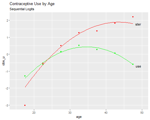
We see that the two quadratics fit reasonably well, except for overestimating the probability of sterilization among contraceptive users at ages 15 to 19, a problem similar to that noted in the multinomial logit model. We could easily remedy this deficiency by adding a dummy variable for teenagers in the second-stage model.
Exercise. In the next section we will study ordered logit models. You may want to try fitting an ordered logit model to this dataset treating the three choices as ordered in terms of contraceptive effectiveness.
Updated fall 2022