
Make sure you read the data as shown in Section 6.1.
> library(haven)
> library(dplyr)
> library(tidyr)
> cuselong <- read_dta("https://grodri.github.io/datasets/elsalvador1985.dta") |>
+   mutate(ageg=as_factor(ageg))
> cuse <- pivot_wider(cuselong, names_from=cuse, values_from=cases)
> names(cuse)[2:4] <- c("ster", "other", "none")
We start with multinomial logit models treating age as a predictor
and contraceptive use as the outcome. R has several functions that can
fit multinomial logit models. We will emphasize the classic
multinom in Venables and Ripley’s nnet package
because it is simple, does everything we need, and is already included
in your R installation. Alternatives include mlogit and
mnlogit; these fit a wider variety of models, but are a bit
harder to use.
Obviously the model that treats age as a factor with 7 levels is
saturated for this data. We can easily obtain the log-likelihood, and
predicted values if we needed them. By default
multinom picks the first response category as the
reference. We take care of that by putting “no method”
first.`’
> library(nnet)
> cuse$Y <- as.matrix(cuse[,c("none","ster","other")])
> msat <- multinom(Y ~ ageg, data=cuse)
# weights: 24 (14 variable)
initial value 3477.107894
iter 10 value 2910.092190
iter 20 value 2872.978246
final value 2872.899103
converged> msatCall:
multinom(formula = Y ~ ageg, data = cuse)
Coefficients:
(Intercept) ageg20-24 ageg25-29 ageg30-34 ageg35-39 ageg40-44 ageg45-49
ster -4.348180 2.7387387 4.0163534 4.6259663 4.39494512 4.2589552 3.649552
other -1.335857 0.2643796 0.5039453 0.3533843 0.01143483 -0.5859748 -1.571018
Residual Deviance: 5745.798
AIC: 5773.798 You could use summary(msat) to obtain standard errors as
well, but we’ll skip those.
Following the notes, we will consider a model with linear and quadratic effects of age. To this end we define the midpoints of age and its square. For consistency with the notes we will not center age before computing the square, although I generally recommend that.
> library(dplyr)
> cuse <- mutate(cuse, age = seq(17.5,47.5,5)[ageg], agesq = age^2)
> cuse$Y = as.matrix(cuse[, c("none", "ster", "other")])
> mlq <- multinom(Y ~ age + agesq, data=cuse)
# weights: 12 (6 variable)
initial value 3477.107894
iter 10 value 2883.272291
final value 2883.136389
converged> summary(mlq)Call:
multinom(formula = Y ~ age + agesq, data = cuse)
Coefficients:
(Intercept) age agesq
ster -12.618330 0.7097288 -0.009732882
other -4.549838 0.2640771 -0.004758144
Std. Errors:
(Intercept) age agesq
ster 0.0003634951 0.006137073 0.0001616953
other 0.0004850755 0.007198081 0.0002166951
Residual Deviance: 5766.273
AIC: 5778.273 > B <- coef(mlq)
> -0.5 * B[,"age"]/B[,"agesq"] ster other
36.46036 27.75000 Compare the parameter estimates with Table 6.2 in the notes. As usual with quadratics, it is easier to plot the results, which we do below. The log-odds of using sterilization rather than no method increase rapidly with age to reach a maximum at 36.5. The log-odds of using a method other than sterilization rather than no method, increase slightly to reach a maximum at age 27.8 and then decline. (The turning points were calculated by setting the derivatives to zero.)
> anova(multinom(Y~1, data=cuse), mlq)# weights: 6 (2 variable)
initial value 3477.107894
final value 3133.450437
convergedLikelihood ratio tests of Multinomial Models
Response: Y
Model Resid. df Resid. Dev Test Df LR stat. Pr(Chi)
1 1 12 6266.901
2 age + agesq 8 5766.273 1 vs 2 4 500.6281 0The model chi-squared, which as usual compares the current and null models, indicates that the hypothesis of no age differences in contraceptive choise is soundly rejected with a chi-squared of 500.6 on 4 d.f. To see where the d.f. come from, note that the current model has six parameters (two quadratics with three parameters each) and the null model of course has only two (the two constants).
To test the goodness of fit of the model we compare it with the model
that treats age as a factor, which is saturated for these data. The
“deviances” reported by multinom’ for these models are
5766.273 and 5745.798. They are calculated as -2logL, where
logL is the individual data log-likelihood. This is why the
“deviance” for the saturated model is not zero. But we can compute
differences among deviances, which are correct.
> anova(mlq, msat) Likelihood ratio tests of Multinomial Models
Response: Y
Model Resid. df Resid. Dev Test Df LR stat. Pr(Chi)
1 age + agesq 8 5766.273
2 ageg 0 5745.798 1 vs 2 8 20.47457 0.008682221> # or "by hand"
> x2 <- deviance(mlq) - deviance(msat)
> data.frame(chisq=x2, pvalue=pchisq(x2, 8, lower.tail=FALSE)) chisq pvalue
1 20.47457 0.008682221The deviance of 20.47 on 8 d.f. is significant at the 1% level, so we have evidence that this model does not fit the data. We explore the lack of fit using a graph.
Let us do Figure 6.1, comparing observed and fitted logits.
We plot observed versus fitted logits, using markers for the observed values and smooth curves for the quadratics.
> library(ggplot2)
> cuse <- mutate(cuse, obs.s = log(ster/none), obs.o = log(other/none))
> fit1 <- function(x) B[1,1] + B[1,2]*x + B[1,3]*x^2
> fit2 <- function(x) B[2,1] + B[2,2]*x + B[2,3]*x^2
> png("fig61r.png", width=500, height=400)
> ggplot(cuse, aes(age, obs.s)) + geom_point() + geom_point(aes(age, obs.o)) +
+       geom_function(fun=fit1, color="green") + geom_function(fun=fit2, color="red") +
+       ggtitle("Contraceptive Use by Age") + ylab("log-odds (no method as baseline)") +
+   annotate(geom="text", x=48, y=fit1(48)-.2, label="ster", color="green") +
+   annotate(geom="text", x=48, y=fit2(48)-.2, label="other", color="red")
>     dev.off()
png
2 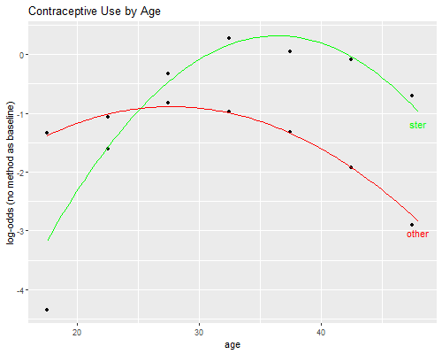
The graph suggests that most of the lack of fit comes from overestimation of the relative odds of being sterilized compared to using no method at ages 15-19. Adding a dummy for this age group confirms the result:
> cuse <- mutate(cuse, age1519 = ageg=="15-19")
> md <- multinom(Y ~ age + agesq + age1519, data=cuse)
# weights: 15 (8 variable)
initial value 3477.107894
iter 10 value 2880.318358
final value 2878.946949
converged> anova(md, msat)Likelihood ratio tests of Multinomial Models
Response: Y
Model Resid. df Resid. Dev Test Df LR stat. Pr(Chi)
1 age + agesq + age1519 6 5757.894
2 ageg 0 5745.798 1 vs 2 6 12.09569 0.05986779The deviance is now only 12.10 on 6 d.f., so we pass the goodness of fit test. (We really didn’t need the dummy in the equation for other methods, so the gain comes from just one d.f.)
An important caveat with multinomial logit models is that we are modeling odds or relative probabilities, and it is always possible for the odds of one category to increase while the probability of that category declines, simply because the odds of another category increase more. To examine this possibility one can always compute predicted probabilities.
We pursue these issues at greater length in a discussion of the interpretation of multinomial logit coefficients, including the calculation of continuous and discrete marginal effects, in an analysis available here.
Updated fall 2022