
This unit illustrates the use of Poisson regression for modeling count data.
We will use the data from Fiji on children ever born that appear on Table 4.1 of the lecture notes. The data are available in the datasets section in both plain text and Stata formats. We will read the Stata file:
> library(haven)
> ceb <- read_dta("https://grodri.github.io/datasets/ceb.dta")
> head(ceb)
# A tibble: 6 × 7
i dur res educ mean var n
<dbl> <dbl+lbl> <dbl+lbl> <dbl+lbl> <dbl> <dbl> <dbl>
1 1 1 [0-4] 1 [Suva] 1 [None] 0.5 1.14 8
2 2 1 [0-4] 1 [Suva] 2 [Lower primary] 1.14 0.730 21
3 3 1 [0-4] 1 [Suva] 3 [Upper primary] 0.900 0.670 42
4 4 1 [0-4] 1 [Suva] 4 [Secondary+] 0.730 0.480 51
5 5 1 [0-4] 2 [Urban] 1 [None] 1.17 1.06 12
6 6 1 [0-4] 2 [Urban] 2 [Lower primary] 0.850 1.59 27The file has 70 observations, one for each cell in the table. Each observation has a sequence number, numeric codes for marriage duration, residence and education, the mean and variance of children ever born, and the number of women in the cell.
We start by doing Figure 4.1, plotting the cell variances versus the cell means using a log-log-scale for cell with at least 20 cases.
> library(ggplot2)Use suppressPackageStartupMessages() to eliminate package startup messages> library(dplyr)
> ceb20 <- filter(ceb, n > 20)
> f <- function(x) x
> png(file="c4fig1r.png", height=400, width=600)
> ggplot(ceb20, aes(mean, var)) + geom_point() +
+ geom_function(fun=f) + coord_trans(x="log", y="log") +
+ ggtitle("Figure 4.1. Mean-Variance Relationship",
+ subtitle="Children Ever Born in Fiji, 1976")
> dev.off()png
2 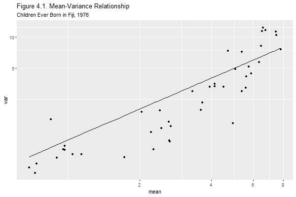
Clearly the variance increases with the mean. Most of the points lie below the 45 degree line, indicating that the variance is not exactly equal to the mean. Still, the assumption of proportionality brings us much closer to the data than the assumption of constant variance.
The dataset does not have information about the number of children ever born (CEB) to each woman, but it turns out that we can still model the mean by working with the cell totals and introducing the log of the number of women in the cell as an offset.
If the number of CEB to one woman in a given cell is a Poisson random variable with mean (and variance) \(\mu\), then the number born to all n women in that cell is a Poisson r.v. with mean (and variance) \(n\mu\). The log of the expected sum is \(\log(n) + \log(\mu)\), and consists of a known offset plus the quantity we are interested in modeling. See the notes for further details
We therefore start by computing the outcome, the total CEB in each
cell, and the offset. We also make sure the discrete variables read as
“labeled” by haven are treated as factors.
> ceb <- mutate(ceb, y = round(mean * n), os = log(n),
+ dur=as_factor(dur), res=as_factor(res), educ=as_factor(educ))We are ready to fit the null model, which has an offset but no predictors.
> m0 <- glm(y ~ 1, family=poisson, offset=os, data=ceb)
> m0
Call:  glm(formula = y ~ 1, family = poisson, data = ceb, offset = os)

Coefficients:
(Intercept)
      1.376

Degrees of Freedom: 69 Total (i.e. Null);  69 Residual
Null Deviance:      3732
Residual Deviance: 3732     AIC: 4163
> exp(coef(m0))(Intercept)
3.960403 > log(weighted.mean(ceb$mean, ceb$n))[1] 1.376369The constant is the log of the mean number of children ever born. Exponentiating we see that the estimated mean is almost four children per woman. The estimate coincides with the sample mean, as we verified by averaging the cell means with the number of women as a frequency weight.
The deviance of 3,732 on 69 d.f. gives a clear indication that the model doesn’t fit the data. The hypothesis that the expected number of CEB is the same for all women regardless of marriage duration, residence and education, is soundly rejected,
Next we fit the three one-factor models, starting with residence:
> mr <- glm(y ~ res, family=poisson, offset=os, data=ceb)
> mr
Call:  glm(formula = y ~ res, family = poisson, data = ceb, offset = os)

Coefficients:
(Intercept)     resUrban     resRural
     1.2046       0.1443       0.2281

Degrees of Freedom: 69 Total (i.e. Null);  67 Residual
Null Deviance:      3732
Residual Deviance: 3659     AIC: 4095
> exp(coef(mr))(Intercept) resUrban resRural
3.335417 1.155219 1.256160 > anova(m0, mr)Analysis of Deviance Table
Model 1: y ~ 1
Model 2: y ~ res
Resid. Df Resid. Dev Df Deviance
1 69 3731.9
2 67 3659.3 2 72.572The estimates show that women in urban and rural areas have on average 16 and 26% more children than women in Suva. The model chi-squared of 73 on 2 d.f. tells us that this model is a significant improvement over the null. The deviance, still in the thousands, tells us that this model is far from fitting the data.
Now for education
> me <- glm(y ~ educ, family=poisson, offset=os, data=ceb)
> me
Call:  glm(formula = y ~ educ, family = poisson, data = ceb, offset = os)

Coefficients:
      (Intercept)  educLower primary  educUpper primary     educSecondary+
           1.6473            -0.2118            -0.6161            -1.2247

Degrees of Freedom: 69 Total (i.e. Null);  66 Residual
Null Deviance:      3732
Residual Deviance: 2661     AIC: 3098
> exp(coef(me)) (Intercept) educLower primary educUpper primary educSecondary+
5.1928251 0.8091371 0.5400718 0.2938527 > anova(m0, me)Analysis of Deviance Table
Model 1: y ~ 1
Model 2: y ~ educ
Resid. Df Resid. Dev Df Deviance
1 69 3731.9
2 66 2661.0 3 1070.8The estimates show that the number of CEB declines substantially with education. Women with secondary education or more have 71% fewer children than women with no education (or only 29% as many). The educational differential is highly significant, but this model doesn’t fit the data.
Finally, here’s duration:
> md <- glm(y ~ dur, family=poisson, offset=os, data=ceb)
> md
Call:  glm(formula = y ~ dur, family = poisson, data = ceb, offset = os)

Coefficients:
(Intercept)       dur5-9     dur10-14     dur15-19     dur20-24       dur25+
    -0.1036       1.0449       1.4449       1.7068       1.8775       2.0789

Degrees of Freedom: 69 Total (i.e. Null);  64 Residual
Null Deviance:      3732
Residual Deviance: 166.1    AIC: 607.5
> exp(coef(md))(Intercept) dur5-9 dur10-14 dur15-19 dur20-24 dur25+
0.9015817 2.8430759 4.2416297 5.5110572 6.5369748 7.9953104 > anova(m0, md)Analysis of Deviance Table
Model 1: y ~ 1
Model 2: y ~ dur
Resid. Df Resid. Dev Df Deviance
1 69 3731.9
2 64 166.1 5 3565.8Not surprisingly, the number of CEB is much higher for women who have been married longer. This is by far the most important predictor of CEB, with a chi-squared of 3,566 on just 5 d.f. In fact, a demographer wouldn’t even have looked at models that did not include a control for duration of marriage. It’s nice to see that Poisson regression can uncover the obvious :) Note that this model still doesn’t fit the data.
The deviances given in this section are pretty close to the deviances in Table 4.3 of the notes. You will notice small differences due to the use of different rounding procedures. In the notes we multiplied the mean CEB by the number of women and retained a few decimals. Here we rounded the total number of CEB to the nearest integer. If you omit the rounding you will reproduce the results in the notes exactly.
We now consider models that take two of the three factors into account. Following the notes we consider only models that include duration of marriage, an essential control when we study cumulative fertility. This leaves two models with main effects of two factors, and another two models that add one interaction.
Because we are only interested in deviances I will run the estimation commands quietly.
So here are the additive models
> mdr <- glm(y ~ dur + res, family=poisson, offset=os, data=ceb)
> deviance(mdr)
[1] 120.6804> mde <- glm(y ~ dur + educ, family=poisson, offset=os, data=ceb)
> deviance(mde)[1] 100.1917And here are the models with one interaction
> mdxr <- glm(y ~ dur * res, family=poisson, offset=os, data=ceb)
> deviance(mdxr)
[1] 108.8965> mdxe <- glm(y ~ dur * educ, family=poisson, offset=os, data=ceb)
> deviance(mdxe) [1] 84.53047The best fit so far is the model that includes duration and education, but it exhibits significant lack of fit with a chi-squared of 84.5 on 46 d.f.
We are now ready to look at models that include all three factors. We start with the additive model.
> mder <- glm(y ~ dur + res + educ, family=poisson, offset=os, data=ceb)
> summary(mder)
Call:
glm(formula = y ~ dur + res + educ, family = poisson, data = ceb,
    offset = os)

Deviance Residuals:
    Min       1Q   Median       3Q      Max
-2.2960  -0.6641   0.0725   0.6336   3.6782

Coefficients:
                  Estimate Std. Error z value Pr(>|z|)
(Intercept)       -0.11710    0.05491  -2.132 0.032969 *
dur5-9             0.99693    0.05274  18.902  < 2e-16 ***
dur10-14           1.36940    0.05107  26.815  < 2e-16 ***
dur15-19           1.61376    0.05119  31.522  < 2e-16 ***
dur20-24           1.78491    0.05121  34.852  < 2e-16 ***
dur25+             1.97641    0.05003  39.501  < 2e-16 ***
resUrban           0.11242    0.03250   3.459 0.000541 ***
resRural           0.15166    0.02833   5.353 8.63e-08 ***
educLower primary  0.02297    0.02266   1.014 0.310597
educUpper primary -0.10127    0.03099  -3.268 0.001082 **
educSecondary+    -0.31015    0.05521  -5.618 1.94e-08 ***
---
Signif. codes:  0 '***' 0.001 '**' 0.01 '*' 0.05 '.' 0.1 ' ' 1

(Dispersion parameter for poisson family taken to be 1)

    Null deviance: 3731.852  on 69  degrees of freedom
Residual deviance:   70.665  on 59  degrees of freedom
AIC: 522.14

Number of Fisher Scoring iterations: 4
> exp(coef(mder)) (Intercept) dur5-9 dur10-14 dur15-19
0.8894987 2.7099627 3.9329722 5.0216439
dur20-24 dur25+ resUrban resRural
5.9590510 7.2167534 1.1189812 1.1637648
educLower primary educUpper primary educSecondary+
1.0232387 0.9036856 0.7333373 This model passes the goodness of fit hurdle, with a deviance of 70.67 on 59 d.f. and a corresponding P-value of 0.14, so we have no evidence against this model.
Briefly, the estimates indicate that the number of CEB increases rapidly with marital duration; in each category of residence and education women married 15-19 years have five times as many children as those married less than five years. Women who live in urban and rural areas have 12% and 16% more children than women who live in Suva and have the same marriage duration and education. Finally, more educated women have fewer children, as women with secondary or more education have on average 27% fewer children than women with no education who live in the same type of place of residence and have been married just as long.
We now put the additive model to some “stress tests” by considering all possible interactions.
> models <- c("dur+res*educ","dur*res+educ","dur*educ+res",
+   "(dur+res)*educ","(dur+educ)*res","dur*(res+educ)",
+   "dur*res*educ - dur:res:educ")
> dd <- matrix(0,length(models),2)
> i <- 1
> for(model in models) {
+   formula <- paste("y ~",model)
+   m <- glm(formula, family=poisson, offset=os, data=ceb)
+   dd[i,] <- c(deviance(m), m$df.residual)
+   i <- i+1
+ }
> data.frame(model=models, deviance=round(dd[,1],2), df=dd[,2],
+   pval=round(pchisq(dd[,1],dd[,2],lower.tail=FALSE),4))
model deviance df pval
1 dur+res*educ 59.92 53 0.2391
2 dur*res+educ 57.13 49 0.1986
3 dur*educ+res 54.80 44 0.1274
4 (dur+res)*educ 44.52 38 0.2163
5 (dur+educ)*res 44.31 43 0.4162
6 dur*(res+educ) 42.65 34 0.1467
7 dur*res*educ - dur:res:educ 30.86 28 0.3235These calculations complete Table 4.3 in the notes. I reported the deviances for consistency with the notes, but could just as well have reported likelihood ratio tests comparing each of these models to the additive model. Make sure you know how to use the output to test, for example, whether we need to add a duration by education interaction. It should be clear from the list of deviances that we don’t need to add any of these terms. We conclude that the additive model does a fine job indeed.
It’s important to note that the need for interactions depends exactly on what’s being modeled. Here we used the log link, so all effects are relative. In this scale no interactions are needed. If we used the identity link we would be modeling the actual number of children ever born, and all effects would be absolute. In that scale we would need, at the very least, interactions with duration of marriage. See the notes for further discussion.
Updated fall 2022