The Deviance Table

Let us reproduce Table 3.13, which compares all possible one, two and three-factor models.

There are 19 basic models for these data. Not all of them would be of interest in any given analysis, but for completeness we will fit all except the null and saturated, effectively reproducing Table 3.13 in the notes.

To simplify some of the repetitive tasks required to fit so many models, I’ll create a vector with the right-hand-side formulas, and write a function to fit each model, pasting the response and adding the family and the data frame before calling glm().

> rhs <- c("1","age", "educ", "nomore",
+    "age + educ", "age + nomore", "educ + nomore", 
+    "age * educ", "age * nomore", "educ * nomore", 
+    "age + educ + nomore",
+    "age * educ + nomore", "age * nomore + educ", 
+    "age + educ * nomore", "age * (educ + nomore)", 
+    "educ * (age + nomore)", "(age + educ) * nomore", 
+    "age*educ*nomore - age:educ:nomore")
> mfit <- function(formula) glm(formula, family=binomial, data=cuse)

Now we simply loop, storing the results in a list

> models <- vector("list",length(rhs))
> for(i in 1:length(rhs)) {
+   mf <- as.formula(paste("Y", rhs[i], sep="~"))
+   models[[i]] <- glm(mf, family="binomial", data=cuse)
+ }

Finally I use lapply() to extract the deviances and df, adding the right-hand sides to identify the models. The result is Table 3.13:

> data.frame(
+   model = rhs, 
+   deviance = round(unlist(lapply(models, deviance)), 2),
+   df = unlist(lapply(models, df.residual))
+ )

                               model deviance df
1                                  1   165.77 15
2                                age    86.58 12
3                               educ   165.07 14
4                             nomore    74.10 14
5                         age + educ    80.42 11
6                       age + nomore    36.89 11
7                      educ + nomore    73.87 13
8                         age * educ    73.03  8
9                       age * nomore    20.10  8
10                     educ * nomore    67.64 12
11               age + educ + nomore    29.92 10
12               age * educ + nomore    23.15  7
13               age * nomore + educ    12.63  7
14               age + educ * nomore    23.02  9
15             age * (educ + nomore)     5.80  4
16             educ * (age + nomore)    13.76  6
17             (age + educ) * nomore    10.82  6
18 age*educ*nomore - age:educ:nomore     2.44  3

Please refer to the notes for various tests based on these models. You should be able to test for net effects of each factor given the other two, test each of the interactions, and test the goodness of fit of each model. We now examine three models of interest.

The Three-factor Additive Model

We now show the coefficients and standard errors for the three-factor additive model, focusing on the net effect of each factor. The gross effects of age and desire or no more children have been shown in earlier sections.

> summary(models[[11]])$coefficients

              Estimate Std. Error    z value     Pr(>|z|)
(Intercept) -1.9661694  0.1720307 -11.429179 2.989214e-30
age25-29     0.3893816  0.1758500   2.214282 2.680938e-02
age30-39     0.9086135  0.1646211   5.519425 3.401115e-08
age40-49     1.1892389  0.2144300   5.546048 2.921980e-08
educ         0.3249947  0.1240355   2.620173 8.788505e-03
nomore       0.8329548  0.1174705   7.090760 1.333778e-12

> exp(coef(models[[11]]))

(Intercept)    age25-29    age30-39    age40-49        educ      nomore 
  0.1399921   1.4760678   2.4808804   3.2845805   1.3840232   2.3001050 

Contraceptive use differs by each of these factors, even when we compare women who fall in the same categories of the other two. For example the odds of using contraception are 38% higher among women with upper primary or more, compared to women with lower primary or less, in the same age group and category of desire for more children.

The deviance of 29.92 on 10 d.f. tells us that this model does not fit the data, so the assumption that logit differences by one variable are the same across categories of the other two is suspect.

The Model with One Interaction Effect

Of the three models with one interaction term, the one that achieves the largest improvement in fit compared to the additive model is the model with an age by no more interaction, where the difference in logits between women who want no more children and those who do varies by age.

The standard reference-cell parametrization can easily be obtained using factor variables:

> summary(models[[13]])$coefficients

                   Estimate Std. Error     z value     Pr(>|z|)
(Intercept)     -1.80317181  0.1801786 -10.0076897 1.410068e-23
age25-29         0.39460393  0.2014504   1.9588147 5.013449e-02
age30-39         0.54666349  0.1984206   2.7550747 5.867873e-03
age40-49         0.57952354  0.3474172   1.6680910 9.529766e-02
nomore           0.06621967  0.3307063   0.2002371 8.412952e-01
educ             0.34064785  0.1257653   2.7086005 6.756764e-03
age25-29:nomore  0.25917997  0.4097504   0.6325314 5.270397e-01
age30-39:nomore  1.11266211  0.3740433   2.9746882 2.932865e-03
age40-49:nomore  1.36167401  0.4843255   2.8114851 4.931338e-03

> b <- coef(models[[13]])
> exp(b[grep("nomore",names(b))])

         nomore age25-29:nomore age30-39:nomore age40-49:nomore 
       1.068461        1.295867        3.042447        3.902721 

Make sure you know how to interpret all of these coefficients. For example the ratio of the odds of using contraception among women who want no more children relative to those who want more in the same category of education is 1.07 among women under age 25, but 3.9 times more (giving an odds ratio of 4.1) among women in their forties.

To aid in interpretation and model criticism we can plot the observed and fitted logits, effectively reproducing Figure 3.4. Because we will need more than one plot, I will encapsulate the calculations in a function `pof()’, for plot observed and fitted.

> library(ggplot2)
> labels = c("nomore/upper", "nomore/lower", "more/upper", "more/lower")
> cuse <- mutate(cuse, agem = c(20, 27.5, 35, 45)[age], obs = log(users/nonusers),
+ code = 5 - 2*nomore - educ, subgroup = factor(code, labels=labels))
> gp <- ggplot(cuse, aes(agem, obs, shape=subgroup, color=subgroup)) + geom_point() +
+   scale_shape_manual(values= c(15, 17, 19, 18)) + xlim(20,50) +
+   theme(legend.position="bottom") + xlab("age") + ylab("logit")
> pof <- function(model, subtitle) {
+   cuse$fit = predict(model, type="link")
+   p <- gp
+   linetypes <- c("solid","dashed","solid","dashed")
+   colors <- c("red", "green","blue","purple")
+   for(i in 1:4) {
+ sg <- filter(cuse, subgroup==labels[i])
+ y <- filter(sg, age=="40-49")$fit
+ lt <- linetypes[i]
+ p = p + geom_line(data=sg, mapping=aes(agem, fit), linetype=lt, color=colors[i]) +
+   annotate("text", x=45.6, y=y, label=labels[i], hjust=0, size=3) +
+   ggtitle("Contraceptive Use by Age, Education and Preferences", subtitle=subtitle)
+   }
+   p
+ }

I first use geom_point to plot the observed logits and save the plot as gp. The function receives a model, adds the fitted logits to the data frame, and plots a line for each subgroup, using annotate to identify the subgroup. I use the same markers as in the notes, but with what I hope is a better legend.

So here’s our first plot

> png("fig34r.png", width=500, height=400)
> pof(models[[13]], "Model with Age by Preferences Interacion")
> dev.off()

png 
  2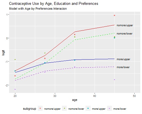 

I often find that interpretation of the interactions is more direct if I combine them with the main effects. Here is the same model showing the difference in logits by desire for more children in each age group, reproducing the results in Table 3.15

> mint <- glm(Y~age + age:nomore + educ, family=binomial, data=cuse)
> exp(coef(mint))

    (Intercept)        age25-29        age30-39        age40-49            educ 
      0.1647754       1.4837964       1.7274796       1.7851877       1.4058581 
  age<25:nomore age25-29:nomore age30-39:nomore age40-49:nomore 
      1.0684614       1.3845839       3.2507371       4.1699068 

We find 34% higher odds of using contraception among women with some education, compared to women with no education in the same age group and category of desire. We also see that the odds of using contraception among women who want no more children are higher than among women who want more children in the same age and category of education, 7% higher under age 25, 38% higher at age 25-29, three times as high for women in their thirties, and four times as high among women in their forties.

This model passes the conventional goodness of fit test and therefore provides a reasonable description of contraceptive use by age, education, and desire for more children.

All Three Two-Factor Interactions

As explained in the notes, there is some evidence that education may interact with the other two variables. The model with all three two-factor interactions provides the best fit, with a deviance of 2.44 on three d.f., but is substantially more complex.

Rather than present parameter estimates, I will reproduce Figure 3.5, which provides some hints on how the model could be simplified. Thanks to our pof command this is now an easy task:

> png("fig35r.png", width=500, height=400)
> pof(models[[18]], "All Two-Factor Interactions")
> dev.off()

png 
  2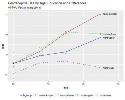 

A picture is indeed worth a thousand words. We see that among women who want no more children, contraceptive use increases almost linearly (in the logit scale) with age, with no differences by education except in the oldest age group, where use flattens for women with no education. Among women who do want more children, contraceptive use is generally lower, and increases more slowly with age; there are some differences by education, and these are higher among older women. There’s also a hint of curvature by age for women with no education who want more children.

A Parsimonious Model

These observations suggest ways to simplify the model. The age interactions are quite simple: the increase with age is steeper among women who want no more children, and the difference by education is larger among women in their forties. Similarly, the educational difference is larger in use for spacing and among older women.

One way to capture these features is to use a quadratic on age, allow the slope (but not the curvature) to vary by desire for more children, and introduce effects of education only for spacing and after age 40 (and thus not for limiting before age 40). To facilitate interpretation of the resulting parameters I center age around 30:

So here is a more parsimonious model

> cuse <- mutate(cuse, agemc = agem - 30, agemcsq=agemc^2,
+   eduspacers = as.numeric(educ==1 & nomore==0),
+   eduforties = as.numeric(educ==1 & age == "40-49"))
> parsi <- glm(Y~ agemc*nomore+ agemcsq+ eduspacers + eduforties,
+   family=binomial, data=cuse)
> parsi

Call:  glm(formula = Y ~ agemc * nomore + agemcsq + eduspacers + eduforties, 
    family = binomial, data = cuse)

Coefficients:
 (Intercept)         agemc        nomore       agemcsq    eduspacers    eduforties  
   -1.339265      0.024755      0.980417     -0.003431      0.432112      0.979816  
agemc:nomore  
    0.058961  

Degrees of Freedom: 15 Total (i.e. Null);  9 Residual
Null Deviance:      165.8 
Residual Deviance: 5.865    AIC: 91.37

This model has only seven parameters and a deviance of 5.9 on 9 d.f., so it is much simpler than the previous model and fits pretty well. Obviously we can’t take the test seriously because we didn’t specify these terms in advance, but the exercise shows how one can simplify a model by capturing its essential features. Before we interpret the coefficients let us check the fitted values

> png("fig35br.png", width=500, height=400)
> pof(parsi, "A Simplified Model")
> dev.off()

png 
  2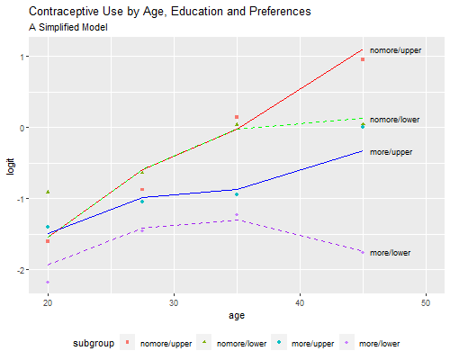 

We see that the model provides almost the same fit as the much more complex model of the previous subsection.

> exp(coef(parsi)["agemc"])

   agemc 
1.025064 

> exp(coef(parsi)[c("nomore","agemc:nomore")])

      nomore agemc:nomore 
    2.665569     1.060734 

> exp(coef(parsi)[c("eduspacers","eduforties")])

eduspacers eduforties 
  1.540508   2.663965 

Returning to the parameter estimates, we see that contraceptive use generally increases with age, with an increment in the odds of about 2.5 percent per year at age 30 (less at younger and older ages, with differences noted below after age 40). Use is much higher among women who want no more children, with an odds ratio of 2.7 at age 30, increasing about six percent per year of age. Women with some education are more likely to use contraception for spacing purposes, with an odds ratio of 1.5, and are also more likely to use for either spacing or limiting after age 40, with an odds ratio of 2.7 (which makes the odds ratio by education for spacers after age 40 just above four).

Alternative model simplifications are given in the notes.

Weighted Individual Data

As promised, we show briefly how one can obtain the same results using a dataset with one row for each combination of predictors and response, with a column indicating the frequency of that combination, effectively simulating individual data.

We will illustrate the equivalence using the model with a main effect of education and an interaction between age and wanting no more children, which we kept as mint.

> cuse2 <- read_dta("https://grodri.github.io/datasets/cuse.dta")
> cuse2 <- mutate(cuse2, age=as_factor(age), educ=as_factor(educ), 
+   nomore=as.numeric(desire==1))
> mintlong <- glm(cuse~age + age:nomore + educ, weights=n, family=binomial, 
+   data=cuse2)
> mint <- glm(Y~age + age:nomore + educ, family=binomial, data=cuse)
> exp(coef(mint))

    (Intercept)        age25-29        age30-39        age40-49            educ 
      0.1647754       1.4837964       1.7274796       1.7851877       1.4058581 
  age<25:nomore age25-29:nomore age30-39:nomore age40-49:nomore 
      1.0684614       1.3845839       3.2507371       4.1699068 

As you can see, the estimates and standard errors are exactly the same as before. The deviance is different because in this dataset the saturated model would have a separate parameter for each woman. We can reproduce the deviance of 12.63 on 7 d.f. given earlier, by computing the difference in deviances (or twice the difference in log-likelihoods) between the model with a three factor interaction and this model:

>    threeway = glm(cuse ~ age*nomore*educ, weights=n, family=binomial, data=cuse2)
>    data.frame( deviance = deviance(mintlong) - deviance(threeway),
+ df = df.residual(mintlong) - df.residual(threeway))

  deviance df
1 12.62955  7

Thus, working with grouped data gives exactly the same estimates as working with individual data, except of course for the deviances. Recall that deviances can be interpreted as goodness of fit tests only with grouped data, but differences in deviances between nested models can always be interpreted as likelihood ratio tests. We discuss how to test goodness of fit with individual data in Section 3.8.

Updated fall 2022