Residuals

Let us start with the residuals. The extractor function residuals() returns raw residuals, and has an optional argument to return other types, but I find it easier to use rstandard() for standardized and rstudent() for studentized residuals. Let us obtain all three:

> ddf <- data.frame( residuals=residuals(m2cg), rstandard=rstandard(m2cg), 
+   rstudent=rstudent(m2cg))

Leverage and Influence

To get the diagonal elements of the hat matrix and Cook’s distance we use the extractor functions hatvalues() and cooks.distance():

> library(dplyr)
> ddf <- mutate(ddf, hat=hatvalues(m2cg), cooks=cooks.distance(m2cg))

We are now ready to print Table 2.29 in the notes.

> ddf

                  residuals    rstandard     rstudent       hat        cooks
Bolivia         -0.83227667 -0.168973754 -0.163754309 0.2616128 2.529026e-03
Brazil           3.42822888  0.657314248  0.645213030 0.1720945 2.245290e-02
Chile            0.44160541  0.083498910  0.080865093 0.1486769 3.044043e-04
Colombia        -1.52718268 -0.291358059 -0.282857589 0.1637904 4.156879e-03
CostaRica        1.28794371  0.242731989  0.235458166 0.1431063 2.459947e-03
Cuba            11.44160541  2.163382852  2.490348474 0.1486769 2.043412e-01
DominicanRep    11.29992007  2.161597338  2.487444785 0.1682585 2.363079e-01
Ecuador        -10.03861524 -1.925295856 -2.126718448 0.1725535 1.932498e-01
ElSalvador       4.65406134  0.895661609  0.889814268 0.1782050 4.348948e-02
Guatemala       -3.49960036 -0.685374906 -0.673572655 0.2064620 3.055405e-02
Haiti            0.02966757  0.006930347  0.006710289 0.4422478 9.520821e-06
Honduras         0.17747027  0.035544869  0.034417531 0.2412746 1.004433e-04
Jamaica         -7.21985927 -1.361728588 -1.402245438 0.1444142 7.824693e-02
Mexico           0.90481996  0.183036697  0.177410357 0.2562359 2.885500e-03
Nicaragua        1.44383484  0.272655282  0.264612794 0.1465179 3.190539e-03
Panama          -5.71205629 -1.076521261 -1.082268869 0.1431063 4.838569e-02
Paraguay        -0.57177112 -0.109628999 -0.106187711 0.1720945 6.245643e-04
Peru            -4.40250346 -0.841096436 -0.833012218 0.1661363 3.523718e-02
TrinidadTobago   1.28794371  0.242731989  0.235458166 0.1431063 2.459947e-03
Venezuela       -2.59323608 -0.575229384 -0.562813507 0.3814295 5.100904e-02

Here is an easy way to find the cases highlighted in Table 2.29, those with standardized or jackknifed residuals greater than 2 in magnitude:

> filter(ddf, abs(rstandard) > 2 | abs(rstudent) > 2)

             residuals rstandard  rstudent       hat     cooks
Cuba          11.44161  2.163383  2.490348 0.1486769 0.2043412
DominicanRep  11.29992  2.161597  2.487445 0.1682585 0.2363079
Ecuador      -10.03862 -1.925296 -2.126718 0.1725535 0.1932498

We will calculate the maximum acceptable leverage, which is 2p/n in general, and then list the cases exceeding that value (if any).

> hatmax = 2*4/20
> filter(ddf, hat > hatmax)

       residuals   rstandard    rstudent       hat        cooks
Haiti 0.02966757 0.006930347 0.006710289 0.4422478 9.520821e-06

We find that Haiti has a lot of leverage, but very little actual influence. Let us list the six most influential countries. I will do this using arrange() with desc() to sort in descending order, and then using subscripts to pick the first 6 rows.

> arrange(ddf, desc(cooks))[1:6,]

              residuals  rstandard   rstudent       hat      cooks
DominicanRep  11.299920  2.1615973  2.4874448 0.1682585 0.23630787
Cuba          11.441605  2.1633829  2.4903485 0.1486769 0.20434122
Ecuador      -10.038615 -1.9252959 -2.1267184 0.1725535 0.19324976
Jamaica       -7.219859 -1.3617286 -1.4022454 0.1444142 0.07824693
Venezuela     -2.593236 -0.5752294 -0.5628135 0.3814295 0.05100904
Panama        -5.712056 -1.0765213 -1.0822689 0.1431063 0.04838569

Turns out that the D.R., Cuba, and Ecuador are fairly influential observations. Try refitting the model without the D.R. to verify what I say on page 57 of the lecture notes.

Residual Plots

On to plots! Here is the standard residual plot in Figure 2.6, produced using the following code:

> library(ggplot2)
> ddf <- mutate(ddf, fitted = fitted(m2cg))
> png("fig26r.png", width=500, height=400)
> ggplot(ddf, aes(fitted, rstudent)) + geom_point() +
+   ggtitle("Figure 2.6: Residual Plot for Ancova Model")   
> dev.off()

png 
  2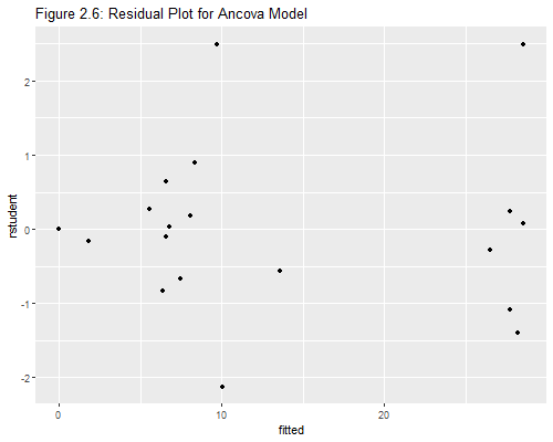 

Exercise: Can you label the points corresponding to Cuba, the D.R. and Ecuador?

Q-Q Plots

Now for that lovely Q-Q-plot in Figure 2.7 of the notes:

> library(ggplot2)
> png("fig27r.png", width=500, height=400)
> ggplot(ddf, aes(sample = rstudent)) +  
+   stat_qq() + geom_abline(intercept=0, slope=1) +
+   ggtitle("Figure 2.7: Q-Q Plot for Residuals of Ancova Model")
> dev.off()

png 
  2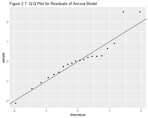 

Wasn’t that easy? The qnorm() function in base R will do this plot, but I used the equivalent stat_qq() in the ggplot2 package. I superimposed a 45 degree line rather than using stata_qq_line(). It is not clear to me how they approximate the rankits, but the calculation seems very close to (i-3/8)/(n+1/4), except for a couple of points on either tail. Of course you can use any approximation you want, albeit at the expense of additional work.

Filliben

I will illustrate the general idea by calculating Filliben’s approximation to the expected order statistics or rankits. After sorting the studentized residuals I use row_number() for the observation number and nrow() for the number of cases.

> N <- nrow(ddf)
> ddf <- arrange(ddf, rstudent) |>
+    mutate(p = (row_number()-0.3175)/(N + 0.365))
> ddf$p[1] <- 1-0.5^(1/N); ddf$p[N] <- 0.5^(1/N)
> ddf <- mutate(ddf, filliben = qnorm(p))
> summarize(ddf, r_rstudent=cor(rstudent,filliben), 
+   r_rstandard=cor(rstandard,filliben))

  r_rstudent r_rstandard
1  0.9517735   0.9655174

The correlation is 0.9518 using jack-knifed residuals, and 0.9655 using standardized residuals. The latter is the value quoted in the notes. Both are above (if barely) the minimum correlation of 0.95 needed to accept normality. I will skip the graph because it looks almost identical to the one produced above.

Updated fall 2022