
We will consider fitting a proportional hazards model of the usual form
\[\tag{7.13}\lambda_i(t|\boldsymbol{x}_i) = \lambda_0(t) \exp \{ \boldsymbol{x}b \}\]under relatively mild assumptions about the baseline hazard \( \lambda_0(t) \).
Consider partitioning duration into \( J \) intervals with cutpoints \( 0 = \tau_0 < \tau_1 < \ldots < \tau_J = \infty \). We will define the \( j \)-th interval as \( [\tau_{j-1},\tau_j) \), extending from the \( (j-1) \)-st boundary to the \( j \)-th and including the former but not the latter.
We will then assume that the baseline hazard is constant within each interval, so that
\[\tag{7.14}\lambda_0(t) = \lambda_j \quad\mbox{for}\: t\:\mbox{in}\quad [\tau_{j-1},\tau_j).\]Thus, we model the baseline hazard \( \lambda_0(t) \) using \( J \) parameters \( \lambda_1,\ldots,\lambda_J \), each representing the risk for the reference group (or individual) in one particular interval. Since the risk is assumed to be piece-wise constant, the corresponding survival function is often called a piece-wise exponential.
Clearly, judicious choice of the cutpoints should allow us to approximate reasonably well almost any baseline hazard, using closely-spaced boundaries where the hazard varies rapidly and wider intervals where the hazard changes more slowly.
Figure 7.2 Approximating a Survival Curve Using a
Piece-wise Constant Hazard Function
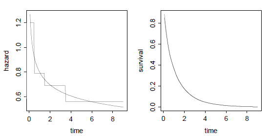
Figure 7.2 shows how a Weibull distribution with \( \lambda=1 \) and \( p=0.8 \) can be approximated using a piece-wise exponential distribution with boundaries at 0.5, 1.5 and 3.5. The left panel shows how the piece-wise constant hazard can follow only the broad outline of the smoothly declining Weibull hazard yet, as shown on the right panel, the corresponding survival curves are indistinguishable.
let us now introduce some covariates in the context of the proportional hazards model in Equation 7.13, assuming that the baseline hazard is piece-wise constant as in Equation 7.14. We will write the model as
\[\tag{7.15}\lambda_{ij} = \lambda_j \exp\{ \boldsymbol{x}_i'\boldsymbol{\beta} \},\]where \( \lambda_{ij} \) is the hazard corresponding to individual \( i \) in interval \( j \), \( \lambda_j \) is the baseline hazard for interval \( j \), and \( \exp\{\boldsymbol{x}_i'\boldsymbol{\beta}\} \) is the relative risk for an individual with covariate values \( \boldsymbol{x}_i \), compared to the baseline, at any given time.
Taking logs, we obtain the additive log-linear model
\[\tag{7.16}\log \lambda_{ij} = \alpha_j + \boldsymbol{x}_i'\boldsymbol{\beta},\]where \( \alpha_j=\log\lambda_j \) is the log of the baseline hazard. Note that the result is a standard log-linear model where the duration categories are treated as a factor. Since we have not included an explicit constant, we do not have to impose restrictions on the \( \alpha_j \). If we wanted to introduce a constant representing the risk in the first interval then we would set \( \alpha_1=0 \), as usual.
The model can be extended to introduce time-varying covariates and time-dependent effects, but we will postpone discussing the details until we study estimation of the simpler proportional hazards model.
Holford (1980) and Laird and Oliver (1981), in papers produced independently and published very close to each other, noted that the piece-wise proportional hazards model of the previous subsection was equivalent to a certain Poisson regression model. We first state the result and then sketch its proof.
Recall that we observe \( t_i \), the total time lived by the \( i \)-th individual, and \( d_i \), a death indicator that takes the value one if the individual died and zero otherwise. We will now define analogous measures for each interval that individual \( i \) goes through. You may think of this process as creating a bunch of pseudo-observations, one for each combination of individual and interval.
First we create measures of exposure. Let \( t_{ij} \) denote the time lived by the \( i \)-th individual in the \( j \)-th interval, that is, between \( \tau_{j-1} \) and \( \tau_j \). If the individual lived beyond the end of the interval, so that \( t_i > \tau_j \), then the time lived in the interval equals the width of the interval and \( t_{ij}=\tau_j-\tau_{j-1} \). If the individual died or was censored in the interval, i.e. if \( \tau_{j-1} < t_i < \tau_j \), then the timed lived in the interval is \( t_{ij}=t_i-\tau_{j-1} \), the difference between the total time lived and the lower boundary of the interval. We only consider intervals actually visited, but obviously the time lived in an interval would be zero if the individual had died before the start of the interval and \( t_i < \tau_{j-1} \).
Now we create death indicators.
Let \( d_{ij} \) take the value one if individual \( i \)
dies in interval \( j \) and zero otherwise.
Let \( j(i) \) indicate the interval where \( t_i \) falls,
i.e. the interval where individual \( i \) died or was censored.
We use functional notation to emphasize that this interval
will vary from one individual to another.
If \( t_i \) falls in interval \( j(i) \), say, then \( d_{ij} \) must be zero
for all \( j Then, the piece-wise exponential model may be fitted to data
by treating the death indicators \( d_{ij} \)’s as if they were independent
Poisson observations with means where \( t_{ij} \) is the exposure time as defined above and
\( \lambda_{ij} \) is the hazard for individual \( i \) in interval
\( j \). Taking logs in this expression, and recalling that the
hazard rates satisfy the proportional hazards model in
Equation 7.15, we obtain where \( \alpha_j=\log\lambda_j \) as before. Thus, the piece-wise exponential proportional hazards model
is equivalent to a Poisson log-linear model for the pseudo
observations, one for each combination of individual and
interval, where the death indicator is the response and the
log of exposure time enters as an offset. It is important to note that we do not assume that the
\( d_{ij} \) have independent Poisson distributions, because they
clearly do not. If individual \( i \) died in interval \( j(i) \),
then it must have been alive in all prior intervals \( j The proof is not hard. Recall from Section 7.2.2
that the contribution of the \( i \)-th individual to the log-likelihood
function has the general form where we have written \( \lambda_i(t) \) for the hazard and
\( \Lambda_i(t) \) for the cumulative hazard that applies to the
\( i \)-th individual at time \( t \). Let \( j(i) \) denote the interval where
\( t_i \) falls, as before. Under the piece-wise exponential model, the first term in the
log-likelihood can be written as using the fact that the hazard is \( \lambda_{ij(i)} \) when \( t_i \) is
in interval \( j(i) \), and that the death indicator \( d_i \) applies
directly to the last interval visited by individual \( i \),
and therefore equals \( d_{j(i)} \). The cumulative hazard in the second term is an integral,
and can be written as a sum as follows where \( t_{ij} \) is the amount of time spent by individual \( i \)
in interval \( j \). To see this point note that we need to integrate
the hazard from 0 to \( t_i \). We split this integral into a sum of
integrals, one for each interval where the hazard is constant.
If an individual lives through an interval, the contribution to
the integral will be the hazard \( \lambda_{ij} \) multiplied by the
width of the interval. If the individual dies or is censored
in the interval, the contribution to the integral will
be the hazard \( \lambda_{ij} \) multiplied by the time elapsed from the
beginning of the interval to the death or censoring time, which is
\( t_i-\tau_{j-1} \). But this is precisely the definition of the
exposure time \( t_{ij} \). One slight lack of symmetry in our results is that the hazard leads
to one term on \( d_{ij(i)}\log \lambda_{ij(i)} \),
but the cumulative hazard
leads to \( j(i) \) terms, one for each interval from \( j=1 \) to \( j(i) \).
However, we know that \( d_{ij}=0 \) for all \( j The fact that the contribution of the individual to the log-likelihood is a
sum of several terms (so the contribution to the likelihood
is a product of several terms) means that we can treat each of the
terms as representing an independent observation. The final step is to identify
the contribution of each pseudo-observation, and we note here that
it agrees, except for a constant, with the likelihood one would
obtain if \( d_{ij} \) had a Poisson distribution with mean
\( \mu_{ij} = t_{ij}\lambda_{ij} \). To see this point write the
Poisson log-likelihood as This expression agrees with the log-likelihood above except for the term
\( d_{ij}\log(t_{ij}) \), but this is a constant depending on the
data and not on the parameters, so it can be ignored from the
point of view of estimation. This completes the proof.\( \Box \) This result generalizes the observation made at the end of Section 7.2.2
noting the relationship between the likelihood for censored exponential
data and the Poisson likelihood. The extension is that instead of having
just one ‘Poisson’ death indicator for each individual, we have one
for each interval visited by each individual. Generating pseudo-observations can substantially increase the
size of the dataset, perhaps to a point where analysis is impractical.
Note, however, that the number of distinct covariate patterns may be modest
even when the total number of pseudo-observations is large.
In this case one can group observations, adding up the measures of
exposure and the death indicators. In this more general setting, we can
define \( d_{ij} \) as the number of deaths and \( t_{ij} \) as the
total exposure time of individuals with
characteristics \( \boldsymbol{x}_i \) in interval \( j \).
As usual with Poisson aggregate models, the estimates, standard
errors and likelihood ratio tests would be exactly the same as
for individual data. Of course, the model deviances would be different,
representing goodness of fit to the aggregate rather than individual
data, but this may be a small price to pay for the convenience of
working with a small number of units. It should be obvious from the previous development that we can
easily accommodate time-varying covariates provided they change
values only at interval boundaries. In creating the pseudo-observations
required to set-up a Poisson log-likelihood, one would normally
replicate the vector of covariates \( \boldsymbol{x}_i \), creating copies
\( \boldsymbol{x}_{ij} \), one for each interval. However, there is nothing
in our development requiring these vectors to be equal. We
can therefore redefine \( \boldsymbol{x}_{ij} \) to represent the values
of the covariates of individual \( i \) in interval \( j \), and
proceed as usual, rewriting the model as Requiring the covariates to change values only at interval
boundaries may seem restrictive, but in practice the model is
more flexible than it might seem at first, because we can
always further split the pseudo observations. For example, if
we wished to accommodate a change in a covariate for individual
\( i \) half-way through interval \( j \), we could split the pseudo-observation
into two, one with the old and one with the new values of the covariates.
Each half would get its own measure of exposure and its own
death indicator, but both would be tagged as belonging to the
same interval, so they would get the same baseline hazard.
All steps in the above proof would still hold. Of course,
splitting observations further increases the size of the dataset,
and there will usually be practical limitations on how far
one can push this approach, even if one uses grouped data.
An alternative is to use simpler indicators such as the mean
value of a covariate in an interval, perhaps lagged to avoid
predicting current hazards using future values of covariates. It turns out that the piece-wise exponential scheme lends
itself easily to the introduction of non-proportional hazards
or time-varying effects, provided again that we let the effects
vary only at interval boundaries. To fix ideas, suppose we have a single predictor taking the
value \( x_{ij} \) for individual \( i \) in interval \( j \).
Suppose further that this predictor is a dummy variable, so its
possible values are one and zero. It doesn’t matter for our
current purpose whether the value is fixed for the individual
or changes from one interval to the next. In a proportional hazards model we would write where \( \beta \) represents the effect of the predictor on the
log of the hazard at any given time. Exponentiating, we see
that the hazard when \( x=1 \) is \( \exp\{\beta\} \) times the
hazard when \( x=0 \), and this effect is the same at all times.
This is a simple additive model on duration and the
predictor of interest. To allow for a time-dependent effect of the predictor, we
would write where \( \beta_j \) represents the effect of the predictor on the
hazard during interval \( j \). Exponentiating, we see that
the hazard in interval \( j \) when \( x=1 \) is \( \exp\{\beta_j\} \)
times the hazard in interval \( j \) when \( x=0 \),
so the effect may vary from one interval to the next.
Since the effect of the predictor depends on the interval,
we have a form of interaction between the predictor and
duration, which might be more obvious if we wrote the model as These models should remind you of the analysis of covariance
models of Chapter 2. Here \( \alpha \) plays the role of the
intercept and \( \beta \) the role of the slope. The proportional
hazards model has different intercepts and a common slope,
so it’s analogous to the parallel lines model. The model
with a time-dependent effect has different intercepts and
different slopes, and is analogous to the model with an
interaction. To sum up, we can accommodate non-proportionality of hazards
simply by introducing interactions with duration. Obviously
we can also test the assumption of proportionality of hazards
by testing the significance of the interactions with duration.
We are now ready for an example.7.4.4 Time-varying Covariates
7.4.5 Time-dependent Effects
Math rendered by
![]()