
The strategy used in Section 6.2.1 to define logits for multinomial response data, namely nominating one of the response categories as a baseline, is only one of many possible approaches.
An alternative strategy is to define a hierarchy of nested comparisons between two subsets of responses, using an ordinary logit model for each comparison. In terms of the contraceptive use example, we could consider (1) the odds of using some form of contraception, as opposed to none, and (2) the odds of being sterilized among users of contraception. For women aged 15–49 these odds are 1494:1671 (or roughly one to one) and 1005:489 (or roughly two to one).
The hierarchical or nested approach is very attractive if you assume that individuals make their decisions in a sequential fashion. In terms of contraceptive use, for example, women may first decide whether or nor they will use contraception. Those who decide to use then face the choice of a method. This sequential approach may also provide a satisfactory model for the “red/blue bus” choice.
Of course it is also possible that the decision to use contraception would be affected by the types of methods available. If that is the case, a multinomial logit model may be more appropriate.
Figure 6.3 Log-Odds of Contraceptive Use vs. No Use and
Sterilization vs. Other Method, by Age.
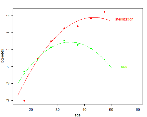
Figure 6.3 shows the empirical log-odds of using any method rather than no method, and of being sterilized rather than using another method among users, by age. Note that contraceptive use increases up to age 35–39 and then declines, whereas the odds of being sterilized among users increase almost monotonically with age.
The data suggest that the hierarchical logits may be modeled as quadratic functions of age, just as we did for the multinomial logits. We will therefore consider the model
\[\tag{6.14}\eta_{ij} = \alpha_j + \beta_j a_i + \gamma_j a_i^2,\]where \( a_i \) is the mid-point of the \( i \)-th age group, \( j=1 \) for the contraceptive use equation and \( j=2 \) for the method choice equation.
An important practical feature of the hierarchical logit model is that the multinomial likelihood factors out into a product of binomial likelihoods, which may then be maximized separately.
I will illustrate using the contraceptive use data with 3 response categories, but the idea is obviously more general. The contribution of the \( i \)-th individual or group to the multinomial likelihood (ignoring constants) has the form
\[\tag{6.15}L_i = \pi_{i1}^{y_{i1}} \pi_{i2}^{y_{i2}} \pi_{i3}^{y_{i3}},\]where the \( \pi_{ij} \) are the probabilities and the \( y_{ij} \) are the corresponding counts of women sterilized, using other methods, and using no methods, respectively.
Multiply and divide this equation by \( (\pi_{i1}+\pi_{i2})^{y_{i1}+y_{i2}} \), which is the probability of using contraception raised to the total number of users of contraception, to obtain
\[\tag{6.16}L_i = \left(\frac{\pi_{i1}}{\pi_{i1}+\pi_{i2}}\right)^{y_{i1}} \left(\frac{\pi_{i2}}{\pi_{i1}+\pi_{i2}}\right)^{y_{i2}} (\pi_{i1}+\pi_{i2})^{y_{i1}+y_{i2}} \pi_{i3}^{y_{i3}}.\]Let \( \rho_{i1} = \pi_{i1} + \pi_{i2} \) denote the probability of using contraception in age group \( i \), and let \( \rho_{i2} = \pi_{i1}/(\pi_{i1}+\pi_{i2}) \) denote the conditional probability of being sterilized given that a woman is using contraception. Using this notation we can rewrite the above equation as
\[\tag{6.17}L_i = \rho_{i2}^{y_{i1}} (1-\rho_{i2})^{y_{i2}} \rho_{i1}^{y_{i1}+y_{i2}} (1-\rho_{i1})^{y_{i3}}.\]The two right-most terms involving the probability of using contraception \( \rho_{i1} \) may be recognized, except for constants, as a standard binomial likelihood contrasting users and non-users. The two terms involving the conditional probability of using sterilization \( \rho_{i2} \) form, except for constants, a standard binomial likelihood contrasting sterilized women with users of other methods. As long as the parameters involved in the two equations are distinct, we can maximize the two likelihoods separately.
In view of this result we turn to Table 6.1 and fit two separate models. Fitting a standard logit model to the contraceptive use contrast (sterilization or other method vs. no method) using linear and quadratic terms on age gives a deviance of 6.12 on four d.f. and the parameter estimates shown in the middle column of Table 6.3. Fitting a similar model to the method choice contrast (sterilization vs. other method, restricted to users) gives a deviance of 10.77 on four d.f. and the parameter estimates shown in the rightmost column of Table 6.3.
The combined deviance is 16.89 on 8 d.f. (\( 6.12 + 10.77 = 16.89 \) and \( 4 + 4 = 8 \)). The associated P-value is 0.031, indicating lack of fit significant at the 5% level. Note, however, that the hierarchical logit model provides a somewhat better fit to these data than the multinomial logit model considered earlier, which had a deviance of 20.5 on the same 8 d.f.
Table 6.3. Parameter Estimates for Hierarchical Logit Model
Fitted to Contraceptive Use Data
| Parameter | Contrast | |
| Use vs. No Use | Ster. vs. Other | |
| Constant | -7.180 | -8.869 |
| Linear | 0.4397 | 0.4942 |
| Quadratic | -0.006345 | -0.005674 |
To look more closely at goodness of fit I used the parameter estimates shown on Table 6.3 to calculate fitted logits and plotted these in Figure 6.3 against the observed logits. The quadratic model seems to do a reasonable job with very few parameters, particularly for overall contraceptive use. The method choice equation overestimates the odds of choosing sterilization for the age group 15–19, a problem shared by the multinomial logit model.
The parameter estimates may also be used to calculate illustrative odds of using contraception or sterilization at various ages. Going through these calculations you will discover that the odds of using some form of contraception increase 80% between ages 25 and 35. On the other hand, the odds of being sterilized among contraceptors increase three and a half times between ages 25 and 35.
With three response categories the only possible set of nested comparisons (aside from a simple reordering of the categories) is
| {1,2} versus {3}, and |
| {1} versus {2}. |
With four response categories there are two main alternatives. One is to contrast
| {1, 2} versus {3, 4}, |
| {1} versus {2}, and |
| {3} versus {4}. |
The other compares
| {1} versus {2, 3, 4}, |
| {2} versus {3, 4}, and |
| {3} versus {4}. |
The latter type of model, where one considers the odds of response \( Y=j \) relative to responses \( Y \ge j \), is known as a continuation ratio model (see Fienberg, 1980), and may be appropriate when the response categories are ordered.
More generally, any set of \( J-1 \) linearly independent contrasts can be selected for modeling, but only orthogonal contrasts lead to a factorization of the likelihood function. The choice of contrasts should in general be based on the logic of the situation.