
We now consider models for the probabilities \( \pi_{ij} \). In particular, we would like to consider models where these probabilities depend on a vector \( \boldsymbol{x}_i \) of covariates associated with the \( i \)-th individual or group. In terms of our example, we would like to model how the probabilities of being sterilized, using another method or using no method at all depend on the woman’s age.
Perhaps the simplest approach to multinomial data is to nominate one of the response categories as a baseline or reference cell, calculate log-odds for all other categories relative to the baseline, and then let the log-odds be a linear function of the predictors.
Typically we pick the last category as a baseline and calculate the odds that a member of group \( i \) falls in category \( j \) as opposed to the baseline as \( \pi_{i1}/\pi_{iJ} \). In our example we could look at the odds of being sterilized rather than using no method, and the odds of using another method rather than no method. For women aged 45–49 these odds are 91:183 (or roughly 1 to 2) and 10:183 (or 1 to 18).
Figure 6.2 Log-Odds of Sterilization vs. No Method and
Other Method vs. No Method, by Age
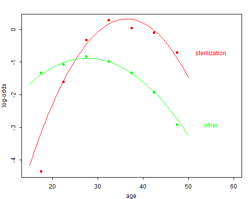
Figure 6.2 shows the empirical log-odds of sterilization and other method (using no method as the reference category) plotted against the mid-points of the age groups. (Ignore for now the solid lines.) Note how the log-odds of sterilization increase rapidly with age to reach a maximum at 30–34 and then decline slightly. The log-odds of using other methods rise gently up to age 25–29 and then decline rapidly.
In the multinomial logit model we assume that the log-odds of each response follow a linear model
\[\tag{6.3}\eta_{ij} = \log\frac{\pi_{ij}}{\pi_{iJ}} = \alpha_j + \boldsymbol{x}_i'\boldsymbol{\beta}_j,\]where \( \alpha_j \) is a constant and \( \boldsymbol{\beta}_j \) is a vector of regression coefficients, for \( j= 1, 2, \ldots, J-1 \). Note that we have written the constant explicitly, so we will assume henceforth that the model matrix \( \boldsymbol{X} \) does not include a column of ones.
This model is analogous to a logistic regression model, except that the probability distribution of the response is multinomial instead of binomial and we have \( J-1 \) equations instead of one. The \( J-1 \) multinomial logit equations contrast each of categories \( 1, 2, \ldots J-1 \) with category \( J \), whereas the single logistic regression equation is a contrast between successes and failures. If \( J=2 \) the multinomial logit model reduces to the usual logistic regression model.
Note that we need only \( J-1 \) equations to describe a variable with \( J \) response categories and that it really makes no difference which category we pick as the reference cell, because we can always convert from one formulation to another. In our example with \( J=3 \) categories we contrast categories 1 versus 3 and 2 versus 3. The missing contrast between categories 1 and 2 can easily be obtained in terms of the other two, since \( \log(\pi_{i1}/\pi_{i2}) = \log(\pi_{i1}/\pi_{i3}) - \log(\pi_{i2}/\pi_{i3}) \).
Looking at Figure 6.2, it would appear that the logits are a quadratic function of age. We will therefore entertain the model
\[\tag{6.4}\eta_{ij} = \alpha_j + \beta_j a_i + \gamma_j a_i^2,\]where \( a_i \) is the midpoint of the \( i \)-th age group and \( j=1,2 \) for sterilization and other method, respectively.
The multinomial logit model may also be written in terms of the original probabilities \( \pi_{ij} \) rather than the log-odds. Starting from r<>q:mlogit and adopting the convention that \( \eta_{iJ} = 0 \), we can write
\[\tag{6.5}\pi_{ij} = \frac{ \exp\{ \eta_{ij} \}} { \sum_{k=1}^J \exp\{ \eta_{ik} \} }.\]for \( j=1, \ldots, J \). To verify this result exponentiate Equation 6.3 to obtain \( \pi_{ij} = \pi_{iJ} \exp\{\eta_{ij}\} \), and note that the convention \( \eta_{iJ}=0 \) makes this formula valid for all \( j \). Next sum over \( j \) and use the fact that \( \sum_j\pi_{ij}=1 \) to obtain \( \pi_{iJ} = 1/\sum_j \exp\{\eta_{ij}\} \). Finally, use this result on the formula for \( \pi_{ij} \).
Note that Equation 6.5 will automatically yield probabilities that add up to one for each \( i \).
Estimation of the parameters of this model by maximum likelihood proceeds by maximization of the multinomial likelihood (6.2) with the probabilities \( \pi_{ij} \) viewed as functions of the \( \alpha_j \) and \( \boldsymbol{\beta}_j \) parameters in Equation 6.3. This usually requires numerical procedures, and Fisher scoring or Newton-Raphson often work rather well. Most statistical packages include a multinomial logit procedure.
In terms of our example, fitting the quadratic multinomial logit model of Equation 6.4 leads to a deviance of 20.5 on 8 d.f. The associated P-value is 0.009, so we have significant lack of fit.
The quadratic age effect has an associated likelihood-ratio \( \chi^2 \) of 500.6 on four d.f. (\( 521.1 - 20.5 = 500.6 \) and \( 12 - 8 = 4 \)), and is highly significant. Note that we have accounted for 96% of the association between age and method choice (\( 500.6/521.1=0.96 \)) using only four parameters.
Table 6.2. Parameter Estimates for Multinomial Logit Model
Fitted to Contraceptive Use Data
| Parameter | Contrast | |
| Ster. vs. None | Other vs. None | |
| Constant | -12.62 | -4.552 |
| Linear | 0.7097 | 0.2641 |
| Quadratic | -0.009733 | -0.004758 |
Table 6.2 shows the parameter estimates for the two multinomial logit equations. I used these values to calculate fitted logits for each age from 17.5 to 47.5, and plotted these together with the empirical logits in Figure 6.2. The figure suggests that the lack of fit, though significant, is not a serious problem, except possibly for the 15–19 age group, where we overestimate the probability of sterilization.
Under these circumstances, I would probably stick with the quadratic model because it does a reasonable job using very few parameters. However, I urge you to go the extra mile and try a cubic term. The model should pass the goodness of fit test. Are the fitted values reasonable?
Multinomial logit models may also be fit by maximum likelihood working with an equivalent log-linear model and the Poisson likelihood. (This section will only be of interest to readers interested in the equivalence between these models and may be omitted at first reading.)
Specifically, we treat the random counts \( Y_{ij} \) as Poisson random variables with means \( \mu_{ij} \) satisfying the following log-linear model
\[\tag{6.6}\log \mu_{ij} = \eta + \theta_i + \alpha^*_j + \boldsymbol{x}_i'\boldsymbol{\beta}^*_j,\]where the parameters satisfy the usual constraints for identifiability. There are three important features of this model:
First, the model includes a separate parameter \( \theta_i \) for each multinomial observation, i.e. each individual or group. This assures exact reproduction of the multinomial denominators \( n_{i} \). Note that these denominators are fixed known quantities in the multinomial likelihood, but are treated as random in the Poisson likelihood. Making sure we get them right makes the issue of conditioning moot.
Second, the model includes a separate parameter \( \alpha^*_j \) for each response category. This allows the counts to vary by response category, permitting non-uniform margins.
Third, the model uses interaction terms \( \boldsymbol{x}_i'\boldsymbol{\beta}^*_j \) to represent the effects of the covariates \( \boldsymbol{x}_i \) on the log-odds of response \( j \). Once again we have a ‘step-up’ situation, where main effects in a logistic model become interactions in the equivalent log-linear model.
The log-odds that observation \( i \) will fall in response category \( j \) relative to the last response category \( J \) can be calculated from Equation 6.6 as
\[\tag{6.7}\log(\mu_{ij}/\mu_{iJ}) = (\alpha^*_j-\alpha^*_J) + \boldsymbol{x}_i'(\boldsymbol{\beta}^*_j-\boldsymbol{\beta}^*_J).\]This equation is identical to the multinomial logit Equation 6.3 with \( \alpha_j=\alpha^*_j-\alpha^*_J \) and \( \boldsymbol{\beta}_j=\boldsymbol{\beta}^*_j-\boldsymbol{\beta}^*_J \). Thus, the parameters in the multinomial logit model may be obtained as differences between the parameters in the corresponding log-linear model. Note that the \( \theta_i \) cancel out, and the restrictions needed for identification, namely \( \eta_{iJ}=0 \), are satisfied automatically.
In terms of our example, we can treat the counts in the original \( 7 \times 3 \) table as 21 independent Poisson observations, and fit a log-linear model including the main effect of age (treated as a factor), the main effect of contraceptive use (treated as a factor) and the interactions between contraceptive use (a factor) and the linear and quadratic components of age:
\[\tag{6.8}\log \mu_{ij} = \eta + \theta_i + \alpha^*_j + \beta^*_j a_i + \gamma^*_j a_i^2\]In practical terms this requires including six dummy variables representing the age groups, two dummy variables representing the method choice categories, and a total of four interaction terms, obtained as the products of the method choice dummies by the mid-point \( a_i \) and the square of the mid-point \( a_i^2 \) of each age group. Details are left as an exercise. (But see the Stata notes.)