
Let us consider a full analysis of the contraceptive use data in Table 3.1, including all three predictors: age, education and desire for more children.
We use three subscripts to reflect the structure of the data, so \( \pi_{ijk} \) is the probability of using contraception in the \( (i,j,k) \)-th group, where \( i=1,2,3,4 \) indexes the age groups, \( j=1,2 \) the levels of education and \( k=1,2 \) the categories of desire for more children.
There are 19 basic models of interest for these data, which are listed for completeness in Table 3.13. Not all of these models would be of interest in any given analysis. The table shows the model in abbreviated notation, the formula for the linear predictor, the deviance and its degrees of freedom. \(\def\ts{\mbox{ }}\)
Table 3.13. Deviance Table for Logit Models of Contraceptive Use
| Model | \(\mbox{logit}(\pi_{ijk})\) | Dev. | d.f. | ||||||
| Null | \(\eta\) | 165.77 | 15 | ||||||
| One Factor | |||||||||
| \(A\)ge | \(\eta\) | \(+\ts\alpha_i\) | 86.58 | 12 | |||||
| \(E\)ducation | \(\eta\) | \(+\ts\beta_j\) | 165.07 | 14 | |||||
| \(D\)esire | \(\eta\) | \(+\ts\gamma_k\) | 74.10 | 14 | |||||
| Two Factors | |||||||||
| \(A +\ts E\) | \(\eta\) | \(+\ts\alpha_i\) | \(+\ts\beta_j\) | 80.42 | 11 | ||||
| \(A +\ts D\) | \(\eta\) | \(+\ts\alpha_i\) | \(+\ts\gamma_k\) | 36.89 | 11 | ||||
| \(E +\ts D\) | \(\eta\) | \(+\ts\beta_j\) | \(+\ts\gamma_k\) | 73.87 | 13 | ||||
| \(A E\) | \(\eta\) | \(+\ts\alpha_i\) | \(+\ts\beta_j\) | \(+\ts{\alpha\beta}_{ij}\) | 73.03 | 8 | |||
| \(A D\) | \(\eta\) | \(+\ts\alpha_i\) | \(+\ts\gamma_k\) | \(+\ts{\alpha\gamma}_{ik}\) | 20.10 | 8 | |||
| \(E D\) | \(\eta\) | \(+\ts\beta_j\) | \(+\ts\gamma_k\) | \(+\ts{\beta\gamma}_{jk}\) | 67.64 | 12 | |||
| Three Factors | |||||||||
| \(A +\ts E +\ts D\) | \(\eta\) | \(+\ts\alpha_i\) | \(+\ts\beta_j\) | \(+\ts\gamma_k\) | 29.92 | 10 | |||
| \(A E +\ts D\) | \(\eta\) | \(+\ts\alpha_i\) | \(+\ts\beta_j\) | \(+\ts\gamma_k\) | \(+\ts{\alpha\beta}_{ij}\) | 23.15 | 7 | ||
| \(A D +\ts E\) | \(\eta\) | \(+\ts\alpha_i\) | \(+\ts\beta_j\) | \(+\ts\gamma_k\) | \(+\ts{\alpha\gamma}_{ik}\) | 12.63 | 7 | ||
| \(A +\ts E D\) | \(\eta\) | \(+\ts\alpha_i\) | \(+\ts\beta_j\) | \(+\ts\gamma_k\) | \(+\ts{\beta\gamma}_{jk}\) | 23.02 | 9 | ||
| \(A E +\ts A D\) | \(\eta\) | \(+\ts\alpha_i\) | \(+\ts\beta_j\) | \(+\ts\gamma_k\) | \(+\ts{\alpha\beta}_{ij}\) | \(+\ts{\alpha\gamma}_{ik}\) | 5.80 | 4 | |
| \(A E +\ts E D\) | \(\eta\) | \(+\ts\alpha_i\) | \(+\ts\beta_j\) | \(+\ts\gamma_k\) | \(+\ts{\alpha\beta}_{ij}\) | \(+\ts{\beta\gamma}_{jk}\) | 13.76 | 6 | |
| \(A D +\ts E D\) | \(\eta\) | \(+\ts\alpha_i\) | \(+\ts\beta_j\) | \(+\ts\gamma_k\) | \(+\ts{\alpha\gamma}_{ik}\) | \(+\ts{\beta\gamma}_{jk}\) | 10.82 | 6 | |
| \(A E +\ts A D +\ts E D\) | \(\eta\) | \(+\ts\alpha_i\) | \(+\ts\beta_j\) | \(+\ts\gamma_k\) | \(+\ts{\alpha\beta}_{ij}\) | \(+\ts{\alpha\gamma}_{ik}\) | \(+\ts{\beta\gamma}_{jk}\) | 2.44 | 3 |
Note first that the null model does not fit the data. The assumption of a common probability of using contraception for all 16 groups of women is clearly untenable.
Next in the table we find the three possible one-factor models. Comparison of these models with the null model provides evidence of significant gross effects of age and desire for more children, but not of education. The likelihood ratio chi-squared tests are 91.7 on one d.f. for desire, 79.2 on three d.f. for age, and 0.7 on one d.f. for education.
Proceeding down the table we find the six possible two-factor models, starting with the additive ones. Here we find evidence of significant net effects of age and desire for more children after controlling for one other factor. For example the test for an effect of desire net of age is a chi-squared of 49.7 on one d.f., obtained by comparing the additive model \( A+D \) on age and desire the one-factor model \( A \) with age alone. Education has a significant effect net of age, but not net of desire for more children. For example the test for the net effect of education controlling for age is 6.2 on one d.f., and follows from the comparison of the \( A+E \) model with \( A \). None of the additive models fits the data, but the closest one to a reasonable fit is \( A+D \).
Next come the models involving interactions between two factors. We use the notation \( E D \) to denote the model with the main effects of \( E \) and \( D \) as well as the \( E \times D \) interaction. Comparing each of these models with the corresponding additive model on the same two factors we obtain a test of the interaction effect. For example comparing the model \( E D \) with the additive model \( E+D \) we can test whether the effect of desire for more children varies with education. Making these comparisons we find evidence of interactions between age and desire for more children (\( \chi^2=16.8 \) on three d.f.), and between education and desire for more children (\( \chi^2=6.23 \) on one d.f.), but not between age and education (\( \chi^2=7.39 \) on three d.f.).
All of the results described so far could be obtained from two-dimensional tables of the type analyzed in the previous sections. The new results begin to appear as we consider the nine possible three-factor models.
The first entry is the additive model \( A+E+D \), with a deviance of 29.9 on ten d.f. This value represents a significant improvement over any of the additive models on two factors. Thus, we have evidence that there are significant net effects of age, education and desire for more children, considering each factor after controlling the other two. For example the test for a net effect of education controlling the other two variables compares the three-factor additive model \( A+E+D \) with the model without education, namely \( A+D \). The difference of 6.97 on one d.f. is significant, with a P-value of 0.008. However, the three-factor additive model does not fit the data.
The next step is to add one interaction between two of the factors. For example the model \( A E+D \) includes the main effects of \( A \), \( E \) and \( D \) and the \( A \times E \) interaction. The interactions of desire for more children with age and with education produce significant gains over the additive model (\( \chi^2=17.3 \) on three d.f. and \( \chi^2=6.90 \) on one d.f., respectively), whereas the interaction between age and education is not significant (\( \chi^2=6.77 \) with three d.f.). These tests for interactions differ from those based on two-factor models in that they take into account the third factor. The best of these models is clearly the one with an interaction between age and desire for more children, \( A D + E \). This is also the first model in our list that actually passes the goodness of fit test, with a deviance of 12.6 on seven d.f.
Does this mean that we can stop our search for an adequate model? Unfortunately, it does not. The goodness of fit test is a joint test for all terms omitted in the model. In this case we are testing for the \( A E \), \( E D \) and \( A E D \) interactions simultaneously, a total of seven parameters. This type of omnibus test lacks power against specific alternatives. It is possible that one of the omitted terms (or perhaps some particular contrast) would be significant by itself, but its effect may not stand out in the aggregate. At issue is whether the remaining deviance of 12.6 is spread out uniformly over the remaining d.f. or is concentrated in a few d.f. If you wanted to be absolutely sure of not missing anything you might want to aim for a deviance below 3.84, which is the five percent critical value for one d.f., but this strategy would lead to over-fitting if followed blindly.
Let us consider the models involving two interactions between two factors, of which there are three. Since the \( A D \) interaction seemed important we restrict attention to models that include this term, so we start from \( A D + E \), the best model so far. Adding the age by education interaction \( A E \) to this model reduces the deviance by 6.83 at the expense of three d.f. A formal test concludes that this interaction is not significant. If we add instead the education by desire interaction \( E D \) we reduce the deviance by only 1.81 at the expense of one d.f. This interaction is clearly not significant. A model-building strategy based on forward selection of variables would stop here and choose \( A D + E \) as the best model on grounds of parsimony and goodness of fit.
An alternative approach is to start with the saturated model and impose progressive simplification. Deleting the three-factor interaction yields the model \( A E + A D + E D \) with three two-factor interactions, which fits the data rather well, with a deviance of just 2.44 on three d.f. If we were to delete the \( A D \) interaction the deviance would rise by 11.32 on three d.f., a significant loss. Similarly, removing the \( A E \) interaction would incur a significant loss of 8.38 on 3 d.f. We can, however, drop the \( E D \) interaction with a non-significant increase in deviance of 3.36 on one d.f. At this point we can also eliminate the \( A E \) interaction, which is no longer significant, with a further loss of 6.83 on three d.f. Thus, a backward elimination strategy ends up choosing the same model as forward selection.
Although you may find these results reassuring, there is a fact that both approaches overlook: the \( A E \) and \( D E \) interactions are jointly significant! The change in deviance as we move from \( A D + E \) to the model with three two-factor interactions is 10.2 on four d.f., and exceeds (although not by much) the five percent critical value of 9.5. This result indicates that we need to consider the more complicated model with all three two-factor interactions. Before we do that, however, we need to discuss parameter estimates for selected models.
Consider first Table 3.14, where we adopt an approach similar to multiple classification analysis to compare the gross and net effects of all three factors. We use the reference cell method, and include the omitted category for each factor (with a dash where the estimated effect would be) to help the reader identify the baseline.
Table 3.14. Gross and Net Effects of Age, Education and Desire
for More Children on Current Use of Contraception
| Variable and | Gross | Net | |
| category | effect | effect | |
| Constant | – | \(-\)1.966 | |
| Age | \(<\)25 | – | – |
| 25–29 | 0.461 | 0.389 | |
| 30–39 | 1.048 | 0.909 | |
| 40–49 | 1.425 | 1.189 | |
| Education | |||
| Lower | – | – | |
| Upper | -0.093 | 0.325 | |
| Desires More | |||
| Yes | – | – | |
| No | 1.049 | 0.833 | |
The gross or unadjusted effects are based on the single-factor models \( A \), \( E \) and \( D \). These effects represent overall differences between levels of each factor, and as such they have descriptive value even if the one-factor models do not tell the whole story. The results can easily be translated into odds ratios. For example not wanting another child is associated with an increase in the odds of using contraception of 185%. Having upper primary or higher education rather than lower primary or less appears to reduce the odds of using contraception by almost 10%.
The net or adjusted effects are based on the three-factor additive model \( A+E+D \). This model assumes that the effect of each factor is the same for all categories of the others. We know, however, that this is not the case—particularly with desire for more children, which has an effect that varies by age—so we have to interpret the results carefully. The net effect of desire for more children shown in Table 3.14 represents an average effect across all age groups and may not be representative of the effect at any particular age. Having said that, we note that desire for no more children has an important effect net of age and education: on the average, it is associated with an increase in the odds of using contraception of 130%.
The result for education is particularly interesting. Having upper primary or higher education is associated with an increase in the odds or using contraception of 38%, compared to having lower primary or less, after we control for age and desire for more children. The gross effect was close to zero. To understand this result bear in mind that contraceptive use in Fiji occurs mostly among older women who want no more children. Education has no effect when considered by itself because in Fiji more educated women are likely to be younger than less educated women, and thus at a stage of their lives when they are less likely to have reached their desired family size, even though they may want fewer children. Once we adjust for their age, calculating the net effect, we obtain the expected association. In this example age is said to act as a suppressor variable, masking the association between education and contraceptive use.
We could easily add columns to Table 3.14 to trace the effects of one factor after controlling for one or both of the other factors. We could, for example, examine the effect of education adjusted for age, the effect adjusted for desire for more children, and finally the effect adjusted for both factors. This type of analysis can yield useful insights into the confounding influences of other variables.
Let us now examine parameter estimates for the model with an age by desire for more children interaction \( A D + E \), where
\[ \mbox{logit}(\pi_{ijk}) = \eta + \alpha_i + \beta_j + \gamma_j + (\alpha\gamma)_{ik}. \]The parameter estimates depend on the restrictions used in estimation. We use the reference cell method, so that \( \alpha_1=\beta_1=\gamma_1=0 \), and \( (\alpha\gamma)_{ik}=0 \) when either \( i=1 \) or \( k=1 \).
In this model \( \eta \) is the logit of the probability of using contraception in the reference cell, that is, for women under 25 with lower primary or less education who want another child. On the other hand \( \beta_2 \) is the effect of upper primary or higher education, compared to lower primary or less, for women in any age group or category of desire for another child. The presence of an interaction makes interpretation of the estimates for age and desire somewhat more involved:
| \(\alpha_i\) | represents the effect of age group \(i\), compared to age \(<\) 25, for women who want more children. |
| \(\gamma_2\) | represents the effect of wanting no more children, compared to desiring more, for women under age 25. |
| \((\alpha\gamma)_{i2}\) | the interaction term, can be interpreted as the additional effect of wanting no more children among women in age group \(i\), compared to women under age 25. |
It is possible to simplify slightly the presentation of the results by combining the interactions with some of the main effects. In the present example, it is convenient to present the estimates of \( \alpha_i \) as the age effects for women who want another child, and to present \( \gamma_2+(\alpha\gamma)_{i2} \) as the effect of not wanting another child for women in age group \( i \).
Calculation of the necessary dummy variables proceeds exactly as in Section 3.5. This strategy leads to the parameter estimates in Table 3.15.
Table 3.15. The Estimates
| Variable | Category | Symbol | Estimate | Std. Err | \(z\)-ratio |
| Constant | \(\eta\) | \(-\)1.803 | 0.180 | \(-\)10.01 | |
| Age | 25–29 | \(\alpha_2\) | 0.395 | 0.201 | 1.96 |
| 30–39 | \(\alpha_3\) | 0.547 | 0.198 | 2.76 | |
| 40–49 | \(\alpha_4\) | 0.580 | 0.347 | 1.67 | |
| Education | Upper | \(\beta_2\) | 0.341 | 0.126 | 2.71 |
| Desires | \(<\)25 | \(\gamma_2\) | 0.066 | 0.331 | 0.20 |
| no more | 25–29 | \(\gamma_2+(\alpha\gamma)_{22}\) | 0.325 | 0.242 | 1.35 |
| at age | 30–39 | \(\gamma_2+(\alpha\gamma)_{32}\) | 1.179 | 0.175 | 6.74 |
| 40–49 | \(\gamma_2+(\alpha\gamma)_{42}\) | 1.428 | 0.354 | 4.04 | |
To aid in interpretation as well as model criticism, Figure 3.4 plots observed logits based on the original data in Table 3.1, and fitted logits based on the model with an age by desire interaction.
Figure 3.4 Logit Model of Contraceptive Use By Age, Education and
Desire for Children, With Age by Desire Interaction
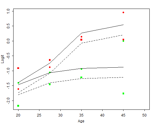
The graph shows four curves tracing contraceptive use by age for groups defined by education and desire for more children. The curves are labelled using \( L \) and \( U \) for lower and upper education, and \( Y \) and \( N \) for desire for more children. The lowest curve labelled \( LY \) corresponds to women with lower primary education or less who want more children, and shows a slight increase in contraceptive use up to age 35–39 and then a small decline. The next curve labelled \( UY \) is for women with upper primary education or more who also want more children. This curve is parallel to the previous one because the effect of education is additive on age. The constant difference between these two curves corresponds to a 41% increase in the odds ratio as we move from lower to upper primary education. The third curve, labelled \( LN \), is for women with lower primary education or less who want no more children. The distance between this curve and the first one represents the effect of wanting no more children at different ages. This effect increases sharply with age, reaching an odds ratio of four by age 40–49. The fourth curve, labelled \( UN \), is for women with upper primary education or more who want no more children. The distance between this curve and the previous one is the effect of education, which is the same whether women want more children or not, and is also the same at every age.
The graph also shows the observed logits, plotted using different symbols for each of the four groups defined by education and desire. Comparison of observed and fitted logits shows clearly the strengths and weaknesses of this model: it does a fairly reasonable job reproducing the logits of the proportions using contraception in each group except for ages 40–49 (and to a lesser extend the group \( < \) 25), where it seems to underestimate the educational differential. There is also some indication that this failure may be more pronounced for women who want more children.
How can we improve the model of the last section? The most obvious solution is to move to the model with all three two-factor interactions, \( AE + AD + ED \), which has a deviance of 2.44 on three d.f. and therefore fits the data extremely well. This model implies that the effect of each factor depends on the levels of the other two, but not on the combination of levels of the other two. Interpretation of the coefficients in this model is not as simple as it would be in an additive model, or in a model involving only one interaction. The best strategy in this case is to plot the fitted model and inspect the resulting curves.
Figure 3.5 Observed and Fitted Logits of Contraceptive Use
Based on Model with Three Two-Factor Interactions
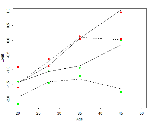
Figure 3.5 shows fitted values based on the more complex model. The plot tells a simple story. Contraceptive use for spacing increases slightly up to age 35 and then declines for the less educated but continues to increase for the more educated. Contraceptive use for limiting increases sharply with age up to age 35 and then levels off for the less educated, but continues to increase for the more educated. The figure shows that the effect of wanting no more children increases with age, and appears to do so for both educational groups in the same way (look at the distance between the LY and LN curves, and between the UY and UN curves). On the other hand, the effect of education is clearly more pronounced at ages 40–49 than at earlier ages, and also seems slightly larger for women who want more children than for those who do not (look at the distance between the LY and UY curves, and between the LN and UN curves).
One can use this knowledge to propose improved models that fit the data without having to use all three two-factor interactions. One approach would note that all interactions with age involve contrasts between ages 40–49 and the other age groups, so one could collapse age into only two categories for purposes of modelling the interactions. A simplified version of this approach is to start from the model \( AD +E \) and add one d.f. to model the larger educational effect for ages 40–49. This can be done by adding a dummy variable that takes the value one for women aged 40–49 who have upper primary or more education. The resulting model has a deviance of 6.12 on six d.f., indicating a good fit. Comparing this value with the deviance of 12.6 on seven d.f. for the \( AD+E \) model, we see that we reduced the deviance by 6.5 at the expense of a single d.f. The model \( AD+AE \) includes all three d.f. for the age by education interaction, and has a deviance of 5.8 on four d.f. Thus, the total contribution of the \( AE \) interaction is 6.8 on three d.f. Our one-d.f. improvement has captured roughly 90% of this interaction.
An alternative approach is to model the effects of education and desire for no more children as smooth functions of age. The logit of the probability of using contraception is very close to a linear function of age for women with upper primary education who want no more children, who could serve as a new reference cell. The effect of wanting more children could be modelled as a linear function of age, and the effect of education could be modelled as a quadratic function of age. Let \( L_{ijk} \) take the value one for lower primary or less education and zero otherwise, and let \( M_{ijk} \) be a dummy variable that takes the value one for women who want more children and zero otherwise. Then the proposed model can be written as
\[ \mbox{logit}(\pi_{ijk}) = \alpha+\beta x_{ijk} + (\alpha_E+\beta_E x_{ijk}+\gamma_E x_{ijk}^2)L_{ijk} + (\alpha_D+\beta_D x_{ijk}) M_{ijk}. \]Fitting this model, which requires only seven parameters, gives a deviance of 7.68 on nine d.f. The only weakness of the model is that it assumes equal effects of education on use for limiting and use for spacing, but these effects are not well-determined. Further exploration of these models is left as an exercise.