
We now consider models involving two predictors, and discuss the binary data analogues of two-way analysis of variance, multiple regression with dummy variables, and analysis of covariance models. An important element of the discussion concerns the key concepts of main effects and interactions.
Consider the distribution of contraceptive use by age and desire for more children, as summarized in Table 3.7. We have a total of eight groups, which will be indexed by a pair of subscripts \( i,j \), with \( i=1,2,3,4 \) referring to the four age groups and \( j=1,2 \) denoting the two categories of desire for more children. We let \( y_{ij} \) denote the number of women using contraception and \( n_{ij} \) the total number of women in age group \( i \) and category \( j \) of desire for more children.
Table 3.7. Contraceptive Use by Age and Desire for More Children
| Age | Desires | Using | Not Using | All |
| \(i\) | \(j\) | \(y_{ij}\) | \(n_{ij}-y_{ij}\) | \(n_{ij}\) |
| \(<\)25 | Yes | 58 | 265 | 323 |
| No | 14 | 60 | 74 | |
| 25–29 | Yes | 68 | 215 | 283 |
| No | 37 | 84 | 121 | |
| 30–39 | Yes | 79 | 230 | 309 |
| No | 158 | 145 | 303 | |
| 40–49 | Yes | 14 | 43 | 57 |
| No | 79 | 58 | 137 | |
| Total | 507 | 1100 | 1607 |
We now analyze these data under the usual assumption of a binomial error structure, so the \( y_{ij} \) are viewed as realizations of independent random variables \( Y_{ij} \sim B(n_{ij}, \pi_{ij}) \).
There are five basic models of interest for the systematic structure of these data, ranging from the null to the saturated model. These models are listed in Table 3.8, which includes the name of the model, a descriptive notation, the formula for the linear predictor, the deviance or goodness of fit likelihood ratio chi-squared statistic, and the degrees of freedom.
Note first that the null model does not fit the data: the deviance of 145.7 on 7 d.f. is much greater than 14.1, the 95-th percentile of the chi-squared distribution with 7 d.f. This result is not surprising, since we already knew that contraceptive use depends on desire for more children and varies by age.
Table 3.8. Deviance Table for Models of Contraceptive Use
by Age (Grouped) and Desire for More Children
| Model | Notation | \(\mbox{logit}(\pi_{ij})\) | Deviance | d.f. |
| Null | \(\phi\) | \(\eta\) | 145.7 | 7 |
| Age | \(A\) | \(\eta + \alpha_i\) | 66.5 | 4 |
| Desire | \(D\) | \(\eta + \beta_j\) | 54.0 | 6 |
| Additive | \(A+D\) | \(\eta + \alpha_i + \beta_j\) | 16.8 | 3 |
| Saturated | \(A D\) | \(\eta+\alpha_i + \beta_j + (\alpha\beta)_{ij}\) | 0 | 0 |
Introducing age in the model reduces the deviance to 66.5 on four d.f. The difference in deviances between the null model and the age model provides a test for the gross effect of age. The difference is 79.2 on three d.f., and is highly significant. This value is exactly the same that we obtained in the previous section, when we tested for an age effect using the data classified by age only. Moreover, the estimated age effects based on fitting the age model to the three-way classification in Table 3.7 would be exactly the same as those estimated in the previous section, and have the property of reproducing exactly the proportions using contraception in each age group.
This equivalence illustrate an important property of binomial models. All information concerning the gross effect of age on contraceptive use is contained in the marginal distribution of contraceptive use by age. We can work with the data classified by age only, by age and desire for more children, by age, education and desire for more children, or even with the individual data. In all cases the estimated effects, standard errors, and likelihood ratio tests based on differences between deviances will be the same.
The deviances themselves will vary, however, because they depend on the context. In the previous section the deviance of the age model was zero, because treating age as a factor reproduces exactly the proportions using contraception by age. In this section the deviance of the age model is 66.5 on four d.f. and is highly significant, because the age model does not reproduce well the table of contraceptive use by both age and preferences. In both cases, however, the difference in deviances between the age model and the null model is 79.2 on three d.f.
The next model in Table 3.8 is the model with a main effect of desire for more children, and has a deviance of 54.0 on six d.f. Comparison of this value with the deviance of the null model shows a gain of 97.1 at the expense of one d.f., indicating a highly significant gross effect of desire for more children. This is, of course, the same result that we obtained in Section 3.3, when we first looked at contraceptive use by desire for more children. Note also that this model does not fit the data, as it own deviance is highly significant.
The fact that the effect of desire for more children has a chi-squared statistic of 91.7 with only one d.f., whereas age gives 79.2 on three d.f., suggests that desire for more children has a stronger effect on contraceptive use than age does. Note, however, that the comparison is informal; the models are not nested, and therefore we cannot construct a significance test from their deviances.
Consider now the two-factor additive model, denoted \( A+D \) in Table 3.8. In this model the logit of the probability of using contraception in age group \( i \) and in category \( j \) of desire for more children is
\[ \mbox{logit}(\pi_{ij}) = \eta + \alpha_i + \beta_j, \]where \( \eta \) is a constant, the \( \alpha_i \) are age effects and the \( \beta_j \) are effects of desire for more children. To avoid redundant parameters we adopt the reference cell method and set \( \alpha_1 = \beta_1 = 0 \). The parameters may then be interpreted as follows:
| \(\eta\) | is the logit of the probability of using contraception for women under 25 who want more children, who serve as the reference cell, |
| \(\alpha_i\) | for \(i=2,3,4\) represents the net effect of ages 25–29, 30–39 and 40–49, compared to women under age 25 in the same category of desire for more children, |
| \(\beta_2\) | represents the net effect of wanting no more children, compared to women who want more children in the same age group. |
The model is additive in the logit scale, in the usual sense that the effect of one variable does not depend on the value of the other. For example, the effect of desiring no more children is \( \beta_2 \) in all four age groups. (This assumption must obviously be tested, and we shall see that it is not consistent with the data.)
The deviance of the additive model is 16.8 on three d.f. With this value we can calculate three different tests of interest, all of which involve comparisons between nested models.
As we move from model \(D\) to \(A+D\) the deviance decreases by 37.2 while we lose three d.f. This statistic tests the hypothesis \(H_0: \alpha_i=0\) for all \(i\), concerning the net effect of age after adjusting for desire for more children, and is highly significant.
As we move from model \(A\) to \(A+D\) we reduce the deviance by 49.7 at the expense of one d.f. This chi-squared statistic tests the hypothesis \(H_0: \beta_2=0\) concerning the net effect of desire for more children after adjusting for age. This value is highly significant, so we reject the hypothesis of no net effects.
Finally, the deviance of 16.8 on three d.f. is a measure of goodness of fit of the additive model: it compares this model with the saturated model, which adds an interaction between the two factors. Since the deviance exceeds 11.3, the one-percent critical value in the chi-squared distribution for three d.f., we conclude that the additive model fails to fit the data.
Table 3.9 shows parameter estimates for the additive model. We show briefly how they would be interpreted, although we have evidence that the additive model does not fit the data.
Table 3.9. Parameter Estimates for Additive Logit Model of
Contraceptive Use by Age (Grouped) and Desire for Children
| Parameter | Symbol | Estimate | Std. Error | \(z\)-ratio | |
| Constant | \(\eta\) | \(-\)1.694 | 0.135 | \(-\)12.53 | |
| Age | 25–29 | \(\alpha_2\) | 0.368 | 0.175 | 2.10 |
| 30–39 | \(\alpha_3\) | 0.808 | 0.160 | 5.06 | |
| 40–49 | \(\alpha_4\) | 1.023 | 0.204 | 5.01 | |
| Desire | No | \(\beta_2\) | 0.824 | 0.117 | 7.04 |
The estimates of the \( \alpha_j \)’s show a monotonic effect of age on contraceptive use. Although there is evidence that this effect may vary depending on whether women desire more children, on average the odds of using contraception among women age 40 or higher are nearly three times the corresponding odds among women under age 25 in the same category of desire for another child.
Similarly, the estimate of \( \beta_2 \) shows a strong effect of wanting no more children. Although there is evidence that this effect may depend on the woman’s age, on average the odds of using contraception among women who desire no more children are more than double the corresponding odds among women in the same age group who desire another child.
We now consider a model which includes an interaction of age and desire for more children, denoted \( A D \) in Table 3.8. The model is
\[ \mbox{logit}(\pi_{ij}) = \eta + \alpha_i + \beta_j + (\alpha\beta)_{ij}, \]where \( \eta \) is a constant, the \( \alpha_i \) and \( \beta_j \) are the main effects of age and desire, and \( (\alpha\beta)_{ij} \) is the interaction effect. To avoid redundancies we follow the reference cell method and set to zero all parameters involving the first cell, so that \( \alpha_1 = \beta_1 = 0 \), \( (\alpha\beta)_{1j} = 0 \) for all \( j \) and \( (\alpha\beta)_{i1} = 0 \) for all \( i \). The remaining parameters may be interpreted as follows:
| \(\eta\) | is the logit of the reference group: women under age 25 who desire more children. |
| \(\alpha_i\) | for \(i=2,3,4\) are the effects of the age groups 25–29, 30–39 and 40–49, compared to ages under 25, for women who want another child. |
| \(\beta_2\) | is the effect of desiring no more children, compared to wanting another child, for women under age 25. |
| \((\alpha\beta)_{i2}\) | for \(i=2,3,4\) is the additional effect of desiring no more children, compared to wanting another child, for women in age group \(i\) rather than under age 25. (This parameter is also the additional effect of age group \(i\), compared to ages under 25, for women who desire no more children rather than those who want more.) |
One way to simplify the presentation of results involving interactions is to combine the interaction terms with one of the main effects, and present them as effects of one factor within categories or levels of the other. In our example, we can combine the interactions \( (\alpha\beta)_{i2} \) with the main effects of desire \( \beta_2 \), so that
| \(\beta_2\) + \((\alpha\beta)_{i2}\) | is the effect of desiring no more children, compared to wanting another child, for women in age group \(i\). |
Of course, we could also combine the interactions with the main effects of age, and speak of age effects which are specific to women in each category of desire for more children. The two formulations are statistically equivalent, but the one chosen here seems demographically more sensible.
To obtain estimates based on this parameterization of the model we have to define the columns of the model matrix as follows. Let \( a_i \) be a dummy variable representing age group \( i \), for \( i=2,3,4 \), and let \( d \) take the value one for women who want no more children and zero otherwise. Then the model matrix \( \boldsymbol{X} \) should have a column of ones to represent the constant or reference cell, the age dummies \( a_2, a_3 \) and \( a_4 \) to represent the age effects for women in the reference cell, and then the dummy \( d \) and the products \( a_2 d, a_3 d \) and \( a_4 d \), to represent the effect of wanting no more children at ages \( <25 \), 25–29, 30–39 and 40–49, respectively. The resulting estimates and standard errors are shown in Table 3.10.
Table 3.10. Parameter Estimates for Model of Contraceptive Use With an
Interaction Between Age (Grouped) and Desire for More Children
| Parameter | Estimate | Std. Error | \(z\)-ratio | |
| Constant | \(-\)1.519 | 0.145 | \(-\)10.481 | |
| Age | 25–29 | 0.368 | 0.201 | 1.832 |
| 30–39 | 0.451 | 0.195 | 2.311 | |
| 40–49 | 0.397 | 0.340 | 1.168 | |
| Desires | \(<\)25 | 0.064 | 0.330 | 0.194 |
| No More | 25–29 | 0.331 | 0.241 | 1.372 |
| at Age | 30–39 | 1.154 | 0.174 | 6.640 |
| 40–49 | 1.431 | 0.353 | 4.057 | |
The results indicate that contraceptive use among women who desire more children varies little by age, increasing up to age 35–39 and then declining somewhat. On the other hand, the effect of wanting no more children increases dramatically with age, from no effect among women below age 25 to an odds ratio of 4.18 at ages 40–49. Thus, in the older cohort the odds of using contraception among women who want no more children are four times the corresponding odds among women who desire more children. The results can also be summarized by noting that contraceptive use for spacing (i.e. among women who desire more children) does not vary much by age, but contraceptive use for limiting fertility (i.e among women who want no more children) increases sharply with age.
Since the model with an age by desire interaction is saturated, we have essentially reproduced the observed data. We now consider whether we could attain a more parsimonious fit by treating age as a variate and desire for more children as a factor, in the spirit of covariance analysis models.
Table 3.11 shows deviances for three models that include a linear effect of age using, as before, the midpoints of the age groups. To emphasize this point we use \( X \) rather than \( A \) to denote age.
Table 3.11. Deviance Table for Models of Contraceptive Use
by Age (Linear) and Desire for More Children
| Model | Notation | \(\mbox{logit}(\pi_{ij})\) | Deviance | d.f. |
| One Line | \(X\) | \(\alpha +\beta x_i\) | 68.88 | 6 |
| Parallel Lines | \(X+D\) | \(\alpha_j+\beta x_i\) | 18.99 | 5 |
| Two Lines | \(X D\) | \(\alpha_j+\beta_j x_i\) | 9.14 | 4 |
The first model assumes that the logits are linear functions of age. This model fails to fit the data, which is not surprising because it ignores desire for more children, a factor that has a large effect on contraceptive use.
The next model, denoted \( X+D \), is analogous to the two-factor additive model. It allows for an effect of desire for more children which is the same at all ages. This common effect is modelled by allowing each category of desire for more children to have its own constant, and results in two parallel lines. The common slope is the effect of age within categories of desire for more children. The reduction in deviance of 39.9 on one d.f. indicates that desire for no more children has a strong effect on contraceptive use after controlling for a linear effect of age. However, the attained deviance of 19.0 on five d.f. is significant, indicating that the assumption of two parallel lines is not consistent with the data.
The last model in the table, denoted \( X D \), includes an interaction between the linear effect of age and desire, and thus allows the effect of desire for more children to vary by age. This variation is modelled by allowing each category of desire for more children to have its own slope in addition to its own constant, and results in two regression lines. The reduction in deviance of 9.9 on one d.f. is a test of the hypothesis of parallelism or common slope \( H_0: \beta_1=\beta_2 \), which is rejected with a P-value of 0.002. The model deviance of 9.14 on four d.f. is just below the five percent critical value of the chi-squared distribution with four d.f., which is 9.49. Thus, we have no evidence against the assumption of two straight lines.
Before we present parameter estimates we need to discuss briefly the choice of parameterization. Direct application of the reference cell method leads us to use four variables: a dummy variable always equal to one, a variable \( x \) with the mid-points of the age groups, a dummy variable \( d \) which takes the value one for women who want no more children, and a variable \( d x \) equal to the product of this dummy by the mid-points of the age groups. This choice leads to parameters representing the constant and slope for women who want another child, and parameters representing the difference in constants and slopes for women who want no more children.
An alternative is to simply report the constants and slopes for the two groups defined by desire for more children. This parameterization can be easily obtained by omitting the constant and using the following four variables: \( d \) and \( 1-d \) to represent the two constants and \( d x \) and \( (1-d)x \) to represent the two slopes. One could, of course, obtain the constant and slope for women who want no more children from the previous parameterization simply by adding the main effect and the interaction. The simplest way to obtain the standard errors, however, is to change parameterization.
In both cases the constants represent effects at age zero and are not very meaningful. To obtain parameters that are more directly interpretable, we can center age around the sample mean, which is 30.6 years. Table 3.12 shows parameter estimates obtained under the two parameterizations discussed above, using the mid-points of the age groups minus the mean.
Table 3.12. Parameter Estimates for Model of Contraceptive Use With an
Interaction Between Age (Linear) and Desire for More Children
| Desire | Age | Symbol | Estimate | Std. Error | \(z\)-ratio |
| More | Constant | \(\alpha_1\) | \(-\)1.1944 | 0.0786 | \(-\)15.20 |
| Slope | \(\beta_1\) | 0.0218 | 0.0104 | 2.11 | |
| No More | Constant | \(\alpha_2\) | \(-\)0.4369 | 0.0931 | \(-\)4.69 |
| Slope | \(\beta_2\) | 0.0698 | 0.0114 | 6.10 | |
| Difference | Constant | \(\alpha_2-\alpha_1\) | 0.7575 | 0.1218 | 6.22 |
| Slope | \(\beta_2-\beta_1\) | 0.0480 | 0.0154 | 3.11 |
Thus, we find that contraceptive use increases with age, but at a faster rate among women who want no more children. The estimated slopes correspond to increases in the odds of two and seven percent per year of age for women who want and do not want more children, respectively. The difference of the slopes is significant by a likelihood ratio test or by Wald’s test, with a \( z \)-ratio of 3.11.
Similarly, the effect of wanting no more children increases with age. The odds ratio around age 30.6—which we obtain by exponentiating the difference in constants–is 2.13, so not wanting more children at this age is associated with a doubling of the odds of using contraception. The difference in slopes of 0.048 indicates that this differential increases five percent per year of age.
The parameter estimates in Table 3.12 may be used to produce fitted logits for each age group and category of desire for more children. In turn, these can be compared with the empirical logits for the original eight groups, to obtain a visual impression of the nature of the relationships studied and the quality of the fit. The comparison appears in Figure 3.3, with the solid line representing the linear age effects (the dotted lines are discussed below). The graph shows clearly how the effect of wanting no more children increases with age (or, alternatively, how age has much stronger effects among limiters than among spacers).
Figure 3.3 Observed and Fitted Logits for Models of Contraceptive Use
With Effects of Age (Linear and Quadratic), Desire for More Children
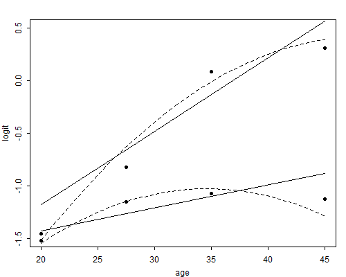
The graph also shows that the assumption of linearity of age effects, while providing a reasonably parsimonious description of the data, is somewhat suspect, particularly at higher ages. We can improve the fit by adding higher-order terms on age. In particular
Introducing a quadratic term on age yields an excellent fit, with a deviance of 2.34 on three d.f. This model consists of two parabolas, one for each category of desire for more children, but with the same curvature.
Adding a quadratic age by desire interaction further reduces the deviance to 1.74 on two d.f. This model allows for two separate parabolas tracing contraceptive use by age, one for each category of desire.
Although the linear model passes the goodness of fit test, the fact that we can reduce the deviance by 6.79 at the expense of one d.f. indicates significant curvature. The dotted line in Figure 3.3 shows the intermediate model, where the curvature by age is the same for the two groups. While the fit is much better, the overall substantive conclusions do not change.