
Let us take a more general look at logistic regression models with a single predictor by considering the comparison of \( k \) groups. This will help us illustrate the logit analogues of one-way analysis of variance and simple linear regression models.
Consider a cross-tabulation of contraceptive use by age, as summarized in Table 3.4. The structure of the data is the same as in the previous section, except that we now have four groups rather than two.
Table 3.4. Contraceptive Use by Age
| Age | Using | Not Using | Total |
| \(i\) | \(y_i\) | \(n_i-y_i\) | \(n_i\) |
| \(<\)25 | 72 | 325 | 397 |
| 25–29 | 105 | 299 | 404 |
| 30–39 | 237 | 375 | 612 |
| 40–49 | 93 | 101 | 194 |
| Total | 507 | 1100 | 1607 |
The analysis of this table proceeds along the same lines as in the two-by-two case. The null model yields exactly the same estimate of the overall logit and its standard error as before. The deviance, however, is now 79.2 on three d.f. This value is highly significant, indicating that the assumption of a common probability of using contraception for the four age groups is not tenable.
Consider now a one-factor model, where we allow each group or level of the discrete factor to have its own logit. We write the model as
\[ \mbox{logit}(\pi_i) = \eta + \alpha_i. \]To avoid redundancy we adopt the reference cell method and set \( \alpha_1=0 \), as before. Then \( \eta \) is the logit of the reference group, and \( \alpha_i \) measures the difference in logits between level \( i \) of the factor and the reference level. This model is exactly analogous to an analysis of variance model. The model matrix \( \boldsymbol{X} \) consists of a column of ones representing the constant and \( k-1 \) columns of dummy variables representing levels two to \( k \) of the factor.
Fitting this model to Table 3.4 leads to the parameter estimates and standard errors in Table 3.5. The deviance for this model is of course zero because the model is saturated: it uses four parameters to model four groups.
Table 3.5. Estimates and Standard Errors for Logit Model
of Contraceptive Use by Age in Groups
| Parameter | Symbol | Estimate | Std. Error | \(z\)-ratio | |
| Constant | \(\eta\) | \(-\)1.507 | 0.130 | \(-\)11.57 | |
| Age | 25–29 | \(\alpha_2\) | 0.461 | 0.173 | 2.67 |
| 30–39 | \(\alpha_3\) | 1.048 | 0.154 | 6.79 | |
| 40–49 | \(\alpha_4\) | 1.425 | 0.194 | 7.35 | |
The baseline logit of \( -1.51 \) for women under age 25 corresponds to odds of 0.22. Exponentiating the age coefficients we obtain odds ratios of 1.59, 2.85 and 4.16. Thus, the odds of using contraception increase by 59% and 185% as we move to ages 25–29 and 30–39, and are quadrupled for ages 40–49, all compared to women under age 25.
All of these estimates can be obtained directly from the frequencies in Table 3.4 in terms of the logits of the observed proportions. For example the constant is \( \mbox{logit}(72/397)=-1.507 \), and the effect for women 25–29 is \( \mbox{logit}(105/404) \) minus the constant.
\( \newcommand{\balpha}{\boldsymbol{\alpha}} \) To test the hypothesis of no age effects we can compare this model with the null model. Since the present model is saturated, the difference in deviances is exactly the same as the deviance of the null model, which was 79.2 on three d.f. and is highly significant. An alternative test of
\[ H_0: \alpha_2 = \alpha_3 = \alpha_4 = 0 \]is based on the estimates and their variance-covariance matrix. Let \( \balpha= (\alpha_2,\alpha_3,\alpha_4)' \). Then
\[ \hat{\balpha} = \left( \begin{array}{r} 0.461\\1.048\\1.425 \end{array} \right) \quad\mbox{and}\quad \hat{\mbox{var}}(\hat{\balpha}) = \left( \begin{array}{rrr} 0.030& 0.017& 0.017\\ 0.017& 0.024& 0.017\\ 0.017& 0.017& 0.038 \end{array} \right), \]and the Wald statistic is
\[ W = \hat{\balpha}' \: \hat{\mbox{var}}^{-1}(\hat{\balpha}) \: \hat{\balpha} = 74.4 \]on three d.f. Again, the Wald test gives results similar to the likelihood ratio test.
Note that the estimated logits in Table 3.5 (and therefore the odds and probabilities) increase monotonically with age. In fact, the logits seem to increase by approximately the same amount as we move from one age group to the next. This suggests that the effect of age may actually be linear in the logit scale.
To explore this idea we treat age as a variate rather than a factor. A thorough exploration would use the individual data with age in single years (or equivalently, a 35 by two table of contraceptive use by age in single years from 15 to 49). However, we can obtain a quick idea of whether the model would be adequate by keeping age grouped into four categories but representing these by the mid-points of the age groups. We therefore consider a model analogous to simple linear regression, where
\[ \mbox{logit}(\pi_i) = \alpha + \beta x_i, \]where \( x_i \) takes the values 20, 27.5, 35 and 45, respectively, for the four age groups. This model fits into our general framework, and corresponds to the special case where the model matrix \( \boldsymbol{X} \) has two columns, a column of ones representing the constant and a column with the mid-points of the age groups, representing the linear effect of age.
Fitting this model gives a deviance of 2.40 on two d.f. , which indicates a very good fit. The parameter estimates and standard errors are shown in Table 3.6. Incidentally, there is no explicit formula for the estimates of the constant and slope in this model, so we must rely on iterative procedures to obtain the estimates.
Table 3.6. Estimates and Standard Errors for Logit Model
of Contraceptive Use with a Linear Effect of Age
| Parameter | Symbol | Estimate | Std. Error | \(z\)-ratio |
| Constant | \(\alpha\) | \(-\)2.673 | 0.233 | \(-\)11.46 |
| Age (linear) | \(\beta\) | 0.061 | 0.007 | 8.54 |
The slope indicates that the logit of the probability of using contraception increases 0.061 for every year of age. Exponentiating this value we note that the odds of using contraception are multiplied by 1.063—that is, increase 6.3%—for every year of age. Note, by the way, that \( e^\beta \approx 1+\beta \) for small \( |\beta| \). Thus, when the logit coefficient is small in magnitude, \( 100\beta \) provides a quick approximation to the percent change in the odds associated with a unit change in the predictor. In this example the effect is 6.3% and the approximation is 6.1%.
To test the significance of the slope we can use the Wald test, which gives a \( z \) statistic of 8.54 or equivalently a chi-squared of 73.9 on one d.f. Alternatively, we can construct a likelihood ratio test by comparing this model with the null model. The difference in deviances is 76.8 on one d.f. Comparing these results with those in the previous subsection shows that we have captured most of the age effect using a single degree of freedom.
Figure 3.2 Observed and Fitted Logits for Model of
Contraceptive Use with a Linear Effect of Age
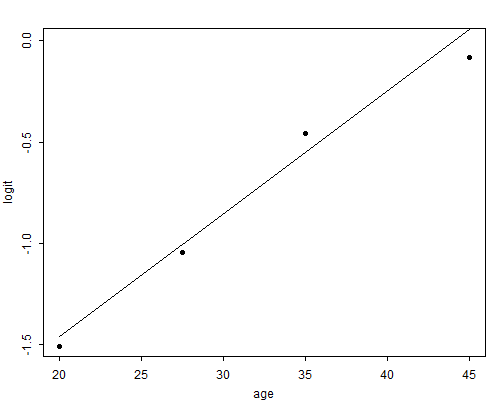
Adding the estimated constant to the product of the slope by the mid-points of the age groups gives estimated logits at each age, and these may be compared with the logits of the observed proportions using contraception. The results of this exercise appear in Figure 3.2. The visual impression of the graph confirms that the fit is quite good. In this example the assumption of linear effects on the logit scale leads to a simple and parsimonious model. It would probably be worthwhile to re-estimate this model using the individual ages.