
The process of statistical modeling involves three distinct stages: formulating a model, fitting the model to data, and checking the model. Often, the third stage suggests a reformulation of the model that leads to a repetition of the entire cycle and, one hopes, an improved model. In this section we discuss techniques that can be used to check the model.
The raw materials of model checking are the residuals \( r_i \) defined as the differences between observed and fitted values
\[\tag{2.23}r_i = y_i - \hat{y}_i,\]where \( y_i \) is the observed response and \( \hat{y_i} = \boldsymbol{x}_i'\hat{\boldsymbol{\beta}} \) is the fitted value for the \( i \)-th unit.
The fitted values may be written in matrix notation as \( \hat{\boldsymbol{y}} = \boldsymbol{X}\hat{\boldsymbol{\beta}} \). Using Equation 2.7 for the m.l.e. of \( \boldsymbol{\beta} \), we can write the fitted values as \( \hat{\boldsymbol{y}} = \boldsymbol{H}\boldsymbol{y} \) where
\[ \boldsymbol{H} = \boldsymbol{X} (\boldsymbol{X}'\boldsymbol{X})^{-1}\boldsymbol{X}'. \]The matrix \( \boldsymbol{H} \) is called the hat matrix because it maps \( y \) into \( y \)-hat. From these results one can show that the fitted values have mean \( E(\hat{\boldsymbol{y}})=\mu \) and variance-covariance matrix \( \mbox{var}(\hat{\boldsymbol{y}})= \boldsymbol{H}\sigma^2 \).
The residuals may be written in matrix notation as \( \boldsymbol{r} = \boldsymbol{y} - \hat{\boldsymbol{y}} \), where \( \boldsymbol{y} \) is the vector of responses and \( \hat{\boldsymbol{y}} \) is the vector of fitted values. Since \( \hat{\boldsymbol{y}}=\boldsymbol{H} \boldsymbol{y} \), we can write the raw residuals as \( \boldsymbol{r} = (\boldsymbol{I}-\boldsymbol{H}) \boldsymbol{y}. \) It is then a simple matter to verify that under the usual second-order assumptions, the residuals have expected value \( \boldsymbol{0} \) and variance-covariance matrix \( \mbox{var}(\boldsymbol{r}) = (\boldsymbol{I}-\boldsymbol{H}) \sigma^2. \) In particular, the variance of the \( i \)-th residual is
\[\tag{2.24}\mbox{var}(r_i) = (1-h_{ii}) \sigma^2,\]where \( h_{ii} \) is the \( i \)-th diagonal element of the hat matrix.
This result shows that the residuals may have different variances even when the original observations all have the same variance \( \sigma^2 \), because the precision of the fitted values depends on the pattern of covariate values.
For models with a constant it can be shown that the value of \( h_{ii} \) is always between \( 1/n \) and \( 1/r \), where \( n \) is the total number of observations and \( r \) is the number of replicates of the \( i \)-th observation (the number of units with the same covariate values as the \( i \)-th unit). In simple linear regression with a constant and a predictor \( x \) we have
\[ h_{ii} = 1/n + \frac{(x_i-\bar{x})^2} {\sum_j(x_j-\bar{x})^2}, \]so that \( h_{ii} \) has a minimum of \( 1/n \) at the mean of \( x \). Thus, the variance of the fitted values is smallest for observations near the mean and increases towards the extremes, as you might have expected. Perhaps less intuitively, this implies that the variance of the residuals is greatest near the mean and decreases as one moves towards either extreme.
Table 2.29 shows raw residuals (and other quantities to be discussed below) for the covariance analysis model fitted to the program effort data. Note that the model underestimates the decline of fertility in both Cuba and the Dominican Republic by a little bit more than eleven percentage points. At the other end of the scale, the model overestimates fertility change in Ecuador by ten percentage points.
Table 2.29. Regression Diagnostics for Analysis of
Covariance Model
of CBR Decline by Social Setting and Program Effort
| Country | Residual | Leverage | Cook's | |||
| \(r_i\) | \(s_i\) | \(t_i\) | \(h_{ii}\) | \(D_i\) | ||
| Bolivia | \(-\)0.83 | \(-\)0.17 | \(-\)0.16 | 0.262 | 0.0025 | |
| Brazil | 3.43 | 0.66 | 0.65 | 0.172 | 0.0225 | |
| Chile | 0.44 | 0.08 | 0.08 | 0.149 | 0.0003 | |
| Colombia | \(-\)1.53 | \(-\)0.29 | \(-\)0.28 | 0.164 | 0.0042 | |
| Costa Rica | 1.29 | 0.24 | 0.24 | 0.143 | 0.0025 | |
| Cuba | 11.44 | 2.16 | 2.49 | 0.149 | 0.2043 | |
| Dominican Rep. | 11.30 | 2.16 | 2.49 | 0.168 | 0.2363 | |
| Ecuador | \(-\)10.04 | \(-\)1.93 | \(-\!\) 2.13 | 0.173 | 0.1932 | |
| El Salvador | 4.65 | 0.90 | 0.89 | 0.178 | 0.0435 | |
| Guatemala | \(-\)3.50 | \(-\)0.69 | \(-\)0.67 | 0.206 | 0.0306 | |
| Haiti | 0.03 | 0.01 | 0.01 | 0.442 | 0.0000 | |
| Honduras | 0.18 | 0.04 | 0.03 | 0.241 | 0.0001 | |
| Jamaica | \(-\)7.22 | \(-\)1.36 | \(-\)1.40 | 0.144 | 0.0782 | |
| Mexico | 0.90 | 0.18 | 0.18 | 0.256 | 0.0029 | |
| Nicaragua | 1.44 | 0.27 | 0.26 | 0.147 | 0.0032 | |
| Panama | \(-\)5.71 | \(-\)1.08 | \(-\)1.08 | 0.143 | 0.0484 | |
| Paraguay | \(-\)0.57 | \(-\)0.11 | \(-\)0.11 | 0.172 | 0.0006 | |
| Peru | \(-\)4.40 | \(-\)0.84 | \(-\)0.83 | 0.166 | 0.0352 | |
| Trinidad-Tobago | 1.29 | 0.24 | 0.24 | 0.143 | 0.0025 | |
| Venezuela | \(-\)2.59 | \(-\)0.58 | \(-\)0.56 | 0.381 | 0.0510 | |
When we compare residuals for different observations we should take into account the fact that their variances may differ. A simple way to allow for this fact is to divide the raw residual by an estimate of its standard deviation, calculating the standardized (or internally studentized) residual
\[\tag{2.25}s_i = \frac{r_i}{ \sqrt{1-h_{ii}} \hat{\sigma} },\]where \( \hat{\sigma} \) is the estimate of the standard deviation based on the residual sum of squares.
Standardized residuals are useful in detecting anomalous observations or outliers. In general, any observation with a standardized residual greater than two in absolute value should be considered worthy of further scrutiny although, as we shall see below, such observations are not necessarily outliers.
Returning to Table 2.29, we see that the residuals for both Cuba and the Dominican Republic exceed two in absolute value, whereas the residual for Ecuador does not. Standardizing the residuals helps assess their magnitude relative to the precision of the estimated regression.
One difficulty with standardized residuals is that they depend on an estimate of the standard deviation that may itself be affected by outliers, which may thereby escape detection.
A solution to this problem is to standardize the \( i \)-th residual using an estimate of the error variance obtained by omitting the \( i \)-th observation. The result is the so-called jack-knifed (or externally studentized, or sometimes just studentized) residual
\[\tag{2.26}t_i = \frac{r_i}{ \sqrt{1-h_{ii}} \hat{\sigma}_{(i)}},\]where \( \hat{\sigma}_{(i)} \) denotes the estimate of the standard deviation obtained by fitting the model without the \( i \)-th observation, and is based on a \( \mbox{RSS} \) with \( n-p-1 \) d.f. Note that the fitted value and the hat matrix are still based on the model with all observations.
You may wonder what would happen if we omitted the \( i \)-th observation not just for purposes of standardizing the residual, but also when estimating the residual itself. Let \( \hat{\boldsymbol{\beta}}_{(i)} \) denote the estimate of the regression coefficients obtained by omitting the \( i \)-th observation. We can combine this estimate with the covariate values of the \( i \)-th observation to calculate a predicted response \( \hat{y}_{(i)} = \boldsymbol{x}_i'\hat{\boldsymbol{\beta}}_{(i)} \) based on the rest of the data. The difference between observed and predicted responses is sometimes called a predictive residual
\[ y_i - \hat{y}_{(i)}. \]Consider now standardizing this residual, dividing by an estimate of its standard deviation. Since the \( i \)-th unit was not included in the regression, \( y_i \) and \( \hat{y}_{(i)} \) are independent. The variance of the predictive residual is
\[ \mbox{var}(y_i-\hat{y}_{(i)}) = (1+ \boldsymbol{x}_i'(\boldsymbol{X}_{(i)}'\boldsymbol{X}_{(i)})^{-1}\boldsymbol{x}_i)\sigma^2, \]where \( \boldsymbol{X}_{(i)} \) is the model matrix without the \( i \)-th row. This variance is estimated replacing the unknown \( \sigma^2 \) by \( \hat{\sigma}^2_{(i)} \), the estimate based on the \( \mbox{RSS} \) of the model omitting the \( i \)-th observation. We are now in a position to calculate a standardized predictive residual
\[\tag{2.27}t_i = \frac{ y_i - \hat{y}_{(i)} } { \sqrt{\hat{\mbox{var}}(y_i-\hat{y}_{(i)})}}.\]The result turns out to be exactly the same as the jack-knifed residual in Equation 2.26 and provides an alternative characterization of this statistic.
At first sight it might appear that jack-knifed residuals require a lot of calculation, as we would need to fit the model omitting each observation in turn. It turns out, however, that there are simple updating formulas that allow direct calculation of regression coefficients and \( \mbox{RSS} \)’s after omitting one observation (see Weisberg, 1985, p. 293). These formulas can be used to show that the jack-knifed residual \( t_i \) is a simple function of the standardized residual \( s_i \)
\[ t_i = s_i \sqrt{ \frac{n-p-1}{n-p-s_i^2} }. \]Note that \( t_i \) is a monotonic function of \( s_i \), so ranking observations by their standardized residuals is equivalent to ordering them by their jack-knifed residuals.
The jack-knifed residuals on Table 2.29 make Cuba and the D.R. stand out more clearly, and suggest that Ecuador may also be an outlier.
The jack-knifed residual can also be motivated as a formal test for outliers. Suppose we start from the model \( \mu_i = \boldsymbol{x}_i'\boldsymbol{\beta} \) and add a dummy variable to allow a location shift for the \( i \)-th observation, leading to the model
\[ \mu_i = \boldsymbol{x}_i'\boldsymbol{\beta} + \gamma z_i, \]where \( z_i \) is a dummy variable that takes the value one for the \( i \)-th observation and zero otherwise. In this model \( \gamma \) represents the extent to which the \( i \)-th response differs from what would be expected on the basis of its covariate values \( \boldsymbol{x}_i \) and the regression coefficients \( \boldsymbol{\beta} \). A formal test of the hypothesis
\[ H_0: \gamma = 0 \]can therefore be interpreted as a test that the \( i \)-th observation follows the same model as the rest of the data (i.e. is not an outlier).
The Wald test for this hypothesis would divide the estimate of \( \gamma \) by its standard error. Remarkably, the resulting \( t \)-ratio,
\[ t_i = \frac{\hat{\gamma}} { \sqrt{\mbox{var}(\hat{\gamma})}} \]on \( n-p-1 \) d.f., is none other than the jack-knifed residual.
This result should not be surprising in light of the previous developments. By letting the \( i \)-th observation have its own parameter \( \gamma \), we are in effect estimating \( \boldsymbol{\beta} \) from the rest of the data. The estimate of \( \gamma \) measures the difference between the response and what would be expected from the rest of the data, and coincides with the predictive residual.
In interpreting the jack-knifed residual as a test for outliers one should be careful with levels of significance. If the suspect observation had been picked in advance then the test would be valid. If the suspect observation has been selected after looking at the data, however, the nominal significance level is not valid, because we have implicitly conducted more than one test. Note that if you conduct a series of tests at the 5% level, you would expect one in twenty to be significant by chance alone.
A very simple procedure to control the overall significance level when you plan to conduct \( k \) tests is to use a significance level of \( \alpha/k \) for each one. A basic result in probability theory known as the Bonferroni inequality guarantees that the overall significance level will not exceed \( \alpha \). Unfortunately, the procedure is conservative, and the true significance level could be considerably less than \( \alpha \).
For the program effort data the jack-knifed residuals have \( 20-4-1=15 \) d.f. To allow for the fact that we are testing 20 of them, we should use a significance level of \( 0.05/20=0.0025 \) instead of \( 0.05 \). The corresponding two-sided critical value of the Student’s \( t \) distribution is \( t_{.99875, 15} = 3.62 \), which is substantially higher than the standard critical value \( t_{.975, 15}=2.13 \). The residuals for Cuba, the D.R. and Ecuador do not exceed this more stringent criterion, so we have no evidence that these countries depart systematically from the model.
Let us return for a moment to the diagonal elements of the hat matrix. Note from Equation 2.24 that the variance of the residual is the product of \( 1-h_{ii} \) and \( \sigma^2 \). As \( h_{ii} \) approaches one the variance of the residual approaches zero, indicating that the fitted value \( \hat{y}_i \) is forced to come close to the observed value \( y_i \). In view of this result, the quantity \( h_{ii} \) has been called the leverage or potential influence of the \( i \)-th observation. Observations with high leverage require special attention, as the fit may be overly dependent upon them.
An observation is usually considered to have high leverage if \( h_{ii} \) exceeds \( 2p/n \), where \( p \) is the number of predictors, including the constant, and \( n \) is the number of observations. This tolerance is not entirely arbitrary. The trace or sum of diagonal elements of \( \boldsymbol{H} \) is \( p \), and thus the average leverage is \( p/n \). An observation is influential if it has more than twice the mean leverage.
Table 2.29 shows leverage values for the analysis of covariance model fitted to the program effort data. With 20 observations and four parameters, we would consider values of \( h_{ii} \) exceeding \( 0.4 \) as indicative of high leverage. The only country that exceeds this tolerance is Haiti, but Venezuela comes close. Haiti has high leverage because it is found rather isolated at the low end of the social setting scale. Venezuela is rather unique in having high social setting but only moderate program effort.
Potential influence is not the same as actual influence, since it is always possible that the fitted value \( \hat{y}_i \) would have come close to the observed value \( y_i \) anyway. Cook proposed a measure of influence based on the extent to which parameter estimates would change if one omitted the \( i \)-th observation. We define Cook's Distance as the standardized difference between \( \hat{\boldsymbol{\beta}}_{(i)} \), the estimate obtained by omitting the \( i \)-th observation, and \( \hat{\boldsymbol{\beta}} \), the estimate obtained using all the data
\[\tag{2.28}D_i = (\hat{\boldsymbol{\beta}}_{(i)} - \hat{\boldsymbol{\beta}})' \: \hat{\mbox{var}}^{-1}(\hat{\boldsymbol{\beta}}) (\hat{\boldsymbol{\beta}}_{(i)} - \hat{\boldsymbol{\beta}}) / p.\]It can be shown that Cook’s distance is also the Euclidian distance (or sum of squared differences) between the fitted values \( \hat{\boldsymbol{y}}_{(i)} \) obtained by omitting the \( i \)-th observation and the fitted values \( \hat{\boldsymbol{y}} \) based on all the data, so that
\[\tag{2.29}D_i = \sum_{j=1}^n ( \hat{y}_{(i)j} - \hat{y}_j ) ^2 / ( p \hat{\sigma}^2).\]This result follows readily from Equation 2.28 if you note that \( \mbox{var}^{-1}(\hat{\boldsymbol{\beta}}) = \boldsymbol{X}'\boldsymbol{X}/\sigma^2 \) and \( \hat{\boldsymbol{y}}_{(i)} = \boldsymbol{X}\hat{\boldsymbol{\beta}}_{(i)} \).
It would appear from this definition that calculation of Cook’s distance requires a lot of work, but the regression updating formulas mentioned earlier simplify the task considerably. In fact, \( D_i \) turns out to be a simple function of the standardized residual \( s_i \) and the leverage \( h_{ii} \),
\[ D_i = s_i^2 \frac{ h_{ii} } { (1-h_{ii}) p }. \]Thus, Cook’s distance \( D_i \) combines residuals and leverages in a single measure of influence.
Values of \( D_i \) near one are usually considered indicative of excessive influence. To provide some motivation for this rule of thumb, note from Equation 2.28 that Cook’s distance has the form \( W/p \), where \( W \) is formally identical to the Wald statistic that one would use to test \( H_0 \): \( \boldsymbol{\beta}=\boldsymbol{\beta}_0 \) if one hypothesized the value \( \hat{\boldsymbol{\beta}}_{(i)} \). Recalling that \( W/p \) has an \( F \) distribution, we see that Cook’s distance is equivalent to the \( F \) statistic for testing this hypothesis. A value of one is close to the median of the \( F \) distribution for a large range of values of the d.f. An observation has excessive influence if deleting it would move this \( F \) statistic from zero to the median, which is equivalent to moving the point estimate to the edge of a 50% confidence region. In such cases it may be wise to repeat the analysis without the influential observation and examine which estimates change as a result.
Table 2.29 shows Cook’s distance for the analysis of covariance model fitted to the program effort data. The D.R., Cuba and Ecuador have the largest indices, but none of them is close to one. To investigate the exact nature of the D.R.’s influence, I fitted the model excluding this country. The main result is that the parameter representing the difference between moderate and weak programs is reduced from 4.14 to 1.89. Thus, a large part of the evidence pointing to a difference between moderate and weak programs comes from the D.R., which happens to be a country with substantial fertility decline and only moderate program effort. Note that the difference was not significant anyway, so no conclusions would be affected.
Note also from Table 2.29 that Haiti, which had high leverage or potential influence, turned out to have no actual influence on the fit. Omitting this country would not alter the parameter estimates at all.
One of the most useful diagnostic tools available to the analyst is the residual plot, a simple scatterplot of the residuals \( r_i \) versus the fitted values \( \hat{y}_i \). Alternatively, one may plot the standardized residuals \( s_i \) or the jack-knifed residuals \( t_i \) versus the fitted values. In all three cases we expect basically a rectangular cloud with no discernible trend or pattern. Figure 2.8 shows a plot of jack-knifed residuals for the analysis of covariance model fitted to the program effort data.
Figure 2.8 Residual Plot for Analysis of Covariance Model
of CBR Decline by Social Setting and Program Effort
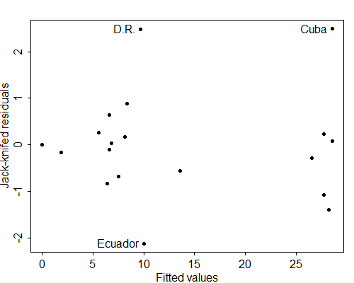
Some of the symptoms that you should be alert for when inspecting residual plots include the following:
Any trend in the plot, such as a tendency for negative residuals at small \(\hat{y}_i\) and positive residuals at large \(\hat{y}_i\). Such a trend would indicate non-linearities in the data. Possible remedies include transforming the response or introducing polynomial terms on the predictors.
Non-constant spread of the residuals, such as a tendency for more clustered residuals for small \(\hat{y}_i\) and more dispersed residuals for large \(\hat{y}_i\). This type of symptom results in a cloud shaped like a megaphone, and indicates heteroscedasticity or non-constant variance. The usual remedy is a transformation of the response.
For examples of residual plots see Weisberg (1985) or Draper and Smith (1966).
A second type of diagnostic aid is the probability plot, a graph of the residuals versus the expected order statistics of the standard normal distribution. This graph is also called a Q-Q Plot because it plots quantiles of the data versus quantiles of a distribution. The Q-Q plot may be constructed using raw, standardized or jack-knifed residuals, although I recommend the latter.
The first step in constructing a Q-Q plot is to order the residuals from smallest to largest, so \( r_{(i)} \) is the \( i \)-th smallest residual. The quantity \( r_{(i)} \) is called an order statistic. The smallest value is the first order statistic and the largest out of \( n \) is the \( n \)-th order statistic.
The next step is to imagine taking a sample of size \( n \) from a standard normal distribution and calculating the order statistics, say \( z_{(i)} \). The expected values of these order statistics are sometimes called rankits. A useful approximation to the \( i \)-th rankit in a sample of size \( n \) is given by
\[ E(\boldsymbol{z}_{(i)}) \approx \Phi^{-1}[(i-3/8)/(n+1/4)] \]where \( \Phi^{-1} \) denotes the inverse of the standard normal distribution function. An alternative approximation proposed by Filliben (1975) uses \( \Phi^{-1}[(i-0.3175)/(n+0.365)] \) except for the first and last rankits, which are estimated as \( \Phi^{-1}(1-0.5^{1/n}) \) and \( \Phi^{-1}(0.5^{1/n}) \), respectively. The two approximations give very similar results.
If the observations come from a normal distribution we would expect the observed order statistics to be reasonably close to the rankits or expected order statistics. In particular, if we plot the order statistics versus the rankits we should get approximately a straight line.
Figure 2.9 shows a Q-Q plot of the jack-knifed residuals from the analysis of covariance model fitted to the program effort data. The plot comes very close to a straight line, except possibly for the upper tail, where we find a couple of residuals somewhat larger than expected.
Figure 2.9 Q-Q Plot of Residuals From
Analysis of Covariance Model
of CBR Decline by Social Setting and Program Effort
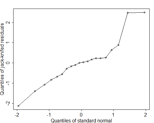
In general, Q-Q plots showing curvature indicate skew distributions, with downward concavity corresponding to negative skewness (long tail to the left) and upward concavity indicating positive skewness. On the other hand, S-shaped Q-Q plots indicate heavy tails, or an excess of extreme values, relative to the normal distribution.
Filliben (1975) has proposed a test of normality based on the linear correlation between the observed order statistics and the rankits and has published a table of critical values. The 5% points of the distribution of \( r \) for \( n=10(10)100 \) are shown below. You would reject the hypothesis of normality if the correlation is less than the critical value. Note than to accept normality we require a very high correlation coefficient.
| \(n\) | 10 | 20 | 30 | 40 | 50 | 60 | 70 | 80 | 90 | 100 |
| \(r\) | .917 | .950 | .964 | .972 | .977 | .980 | .982 | .984 | .985 | .987 |
The Filliben test is closely related to the Shapiro-Francia approximation to the Shapiro-Wilk test of normality. These tests are often used with standardized or jack-knifed residuals, although the fact that the residuals are correlated affects the significance levels to an unknown extent. For the program effort data in Figure 2.9 the Filliben correlation is a respectable 0.966. Since this value exceeds the critical value of 0.950 for 20 observations, we conclude that we have no evidence against the assumption of normally distributed residuals.