
We now consider models where some of the predictors are continuous variates and some are discrete factors. We continue to use the family planning program data, but this time we treat social setting as a variate and program effort as a factor.
Table 2.22 shows the effort data classified into three groups, corresponding to weak (0–4), moderate (5–14) and strong (15+) programs. For each group we list the values of social setting and CBR decline.
Table 2.22. Social Setting Scores and CBR Percent Declines
by Levels of Family Planning Effort
| Family Planning Effort | |||||||
| Weak | Moderate | Strong | |||||
| Setting | Change | Setting | Change | Setting | Change | ||
| 46 | 1 | 68 | 21 | 89 | 29 | ||
| 74 | 10 | 70 | 0 | 77 | 25 | ||
| 35 | 0 | 60 | 13 | 84 | 29 | ||
| 83 | 9 | 55 | 4 | 89 | 40 | ||
| 68 | 7 | 51 | 7 | 87 | 21 | ||
| 74 | 6 | 91 | 11 | 84 | 22 | ||
| 72 | 2 | 84 | 29 | ||||
As usual, we modify our notation to reflect the structure of the data. Let \( k \) denote the number of groups, or levels of the discrete factor, \( n_i \) the number of observations in group \( i \), \( y_{ij} \) the value of the response and \( x_{ij} \) the value of the predictor for the \( j \)-th unit in the \( i \)-th group, with \( j=1,\ldots,n_i \) and \( i=1,\ldots,k \).
We keep the random structure of our model, treating \( y_{ij} \) as a realization of a random variable \( Y_{ij}\sim N(\mu_{ij},\sigma^2) \). To express the dependence of the expected response \( \mu_{ij} \) on a discrete factor we have used an anova model of the form \( \mu_{ij}=\mu+\alpha_i \), whereas to model the effect of a continuous predictor we have used a regression model of the form \( \mu_{ij} = \alpha + \beta x_{ij} \). Combining these two models we obtain the additive analysis of covariance model
\[\tag{2.21}\mu_{ij} = \mu + \alpha_i + \beta x_{ij}.\]This model defines a series of straight-line regressions, one for each level of the discrete factor (you may want to peek at Figure 2.6). These lines have different intercepts \( \mu+\alpha_i \), but a common slope \( \beta \), so they are parallel. The common slope \( \beta \) represents the effects of the continuous variate at any level of the factor, and the differences in intercept \( \alpha_i \) represent the effects of the discrete factor at any given value of the covariate.
The model as defined in Equation 2.21 is not identified: we could add a constant \( \delta \) to each \( \alpha_i \) and subtract it from \( \mu \) without changing any of the expected values. To solve this problem we set \( \alpha_1=0 \), so \( \mu \) becomes the intercept for the reference cell, and \( \alpha_i \) becomes the difference in intercepts between levels \( i \) and one of the factor.
The analysis of covariance model may be obtained as a special case of the general linear model by letting the model matrix \( \boldsymbol{X} \) have a column of ones representing the constant, a set of \( k \) dummy variables representing the levels of the discrete factor, and a column with the values of the continuous variate. The model is not of full column rank because the dummies add up to the constant, so we drop one of them, obtaining the reference cell parametrization. Estimation and testing then follows form the general results in Sections 2.2 and 2.3.
Table 2.23 shows the parameter estimates, standard errors and \( t \)-ratios after fitting the model to the program effort data with setting as a variate and effort as a factor with three levels.
Table 2.23. Parameter Estimates for Analysis of Covariance Model
of CBR Decline by Social Setting and Family Planning Effort
| Parameter | Symbol | Estimate | Std.Error | \(t\)-ratio | |
| Constant | \(\mu\) | \(-\)5.954 | 7.166 | \(-\)0.83 | |
| Effort | moderate | \(\alpha_2\) | 4.144 | 3.191 | 1.30 |
| strong | \(\alpha_3\) | 19.448 | 3.729 | 5.21 | |
| Setting | (linear) | \(\beta\) | 0.1693 | 0.1056 | 1.60 |
The results show that each point in the social setting scale is associated with a further 0.17 percentage points of CBR decline at any given level of effort. Countries with moderate and strong programs show additional CBR declines of 19 and 4 percentage points, respectively, compared to countries with weak programs at the same social setting.
Figure 2.6 Analysis of Covariance Model for CBR Decline
by Social Setting Score and Level of Program Effort
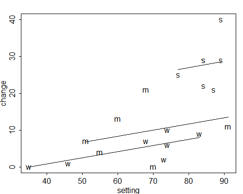
Figure 2.6 depicts the analysis of covariance model in graphical form. We have plotted CBR decline as a function of social setting using the letters w, m and s for weak, moderate and strong programs, respectively. The figure also shows the fitted lines for the three types of programs. The vertical distances between the lines represent the effects of program effort at any given social setting. The common slope represents the effect of setting at any given level of effort.
Fitting the analysis of covariance model to our data gives a \( \mbox{RSS} \) of 525.7 on 16 d.f. (20 observations minus four parameters: the constant, two intercepts and one slope). Combining this result with the \( \mbox{RSS} \)’s for the null model and for the model of Section 2.4 with a linear effect of setting, leads to the hierarchical analysis of variance shown in Table 2.24.
Table 2.24. Hierarchical Anova for Analysis of Covariance Model
of CBR Decline by Social Setting and Family Planning Effort
| Source of | Sum of | Degrees of | Mean | \(F\)- |
| variation | squares | freedom | squared | ratio |
| Setting (linear) | 1201.1 | 1 | 1201.1 | 36.5 |
| Effort\(|\)Setting | 923.4 | 2 | 461.7 | 14.1 |
| Residual | 525.7 | 16 | 32.9 | |
| Total | 2650.2 | 19 |
The most interesting statistic in this table is the \( F \)-test for the net effect of program effort, which is 14.1 on two and 16 d.f. and is highly significant, so we reject the hypothesis \( H_0: \alpha_2=\alpha_3=0 \) of no program effects. Looking at the \( t \)-ratios in Table 2.23 we see that the difference between strong and weak programs is significant, while that between moderate and weak programs is not, confirming our earlier conclusions. The difference between strong and moderate programs, which is not shown in the table, is also significant.
From these results we can calculate proportions of variance explained in the usual fashion. In this example setting explains 45.3% of the variation in CBR declines and program effort explains an additional 34.5%, representing 63.7% of what remained unexplained, for a total of 80.1%. You should be able to translate these numbers into simple, partial and multiple correlation coefficients or ratios.
The estimated net effects of setting and effort based on the analysis of covariance model may be compared with the estimated gross effects based on the simple linear regression model for setting and the one-way analysis of variance model for effort. The results are presented in a format analogous to multiple classification analysis in Table 2.25, where we have used the reference cell method rather than the ‘usual’ restrictions.
Table 2.25. Gross and Net Effects of Social Setting Score
and Level of Family Planning Effort on CBR Decline
| Predictor | Category | Effect | |||
| Gross | Net | ||||
| Setting | (linear) | 0.505 | 0.169 | ||
| Effort | Weak | – | – | ||
| Moderate | 4.33 | 4.14 | |||
| Strong | 22.86 | 19.45 | |||
The effect of social setting is reduced substantially after adjusting for program effort. On the other hand, the effects of program effort, measured by comparing strong and moderate programs with weak ones, are hardly changed after adjustment for social setting.
If interest centers on the effects of program effort, it may be instructive to calculate CBR declines by categories of program effort unadjusted and adjusted for linear effects of setting. To obtain adjusted means we use the fitted model to predict CBR decline with program effort set at the observed values but social setting set at the sample mean, which is 72.1 points. Thus, we calculate expected CBR decline at level \( i \) of effort holding setting constant at the mean as \( \hat{\mu_i} = \hat{\mu} + \hat{\alpha}_i + \hat{\beta}\: 72.1 \). The results are shown in Table 2.26.
Table 2.26. CBR Decline by Family Planning Effort
Before and After Linear Adjustment for Social Setting
| Effort | CBR Decline | |
| Unadjusted | Adjusted | |
| Weak | 5.00 | 6.25 |
| Moderate | 9.33 | 10.40 |
| Strong | 27.86 | 25.70 |
Thus, countries with strong program show on average a 28% decline in the CBR, but these countries tend to have high social settings. If we adjusted linearly for this advantage, we would expect them to show only a 26% decline. Clearly, adjusting for social setting does not change things very much.
Note that the analysis in this sections parallels the results in Section 2.7. The only difference is the treatment of social setting as a discrete factor with three levels or as a continuous variate with a linear effect.
In order to test the assumption of equal slopes in the analysis of covariance model we consider a more general model where
\[\tag{2.22}\mu_{ij} = (\mu + \alpha_i) + (\beta + \gamma_i) x_{ij}.\]In this formulation each of the \( k \) groups has its own intercept \( \mu+\alpha_i \) and its own slope \( \beta+\gamma_i \).
As usual, this model is overparametrized and we introduce the reference cell restrictions, setting \( \alpha_1=\gamma_1=0 \). As a result, \( \mu \) is the constant and \( \beta \) is the slope for the reference cell, \( \alpha_i \) and \( \gamma_i \) are the differences in intercept and slope, respectively, between level \( i \) and level one of the discrete factor. (An alternative is to drop \( \mu \) and \( \beta \), so that \( \alpha_i \) is the constant and \( \gamma_i \) is the slope for group \( i \). The reference cell method, however, extends more easily to models with more than one discrete factor.)
The parameter \( \alpha_i \) may be interpreted as the effect of level \( i \) of the factor, compared to level one, when the covariate is zero. (This value will not be of interest if zero is not in the range of the data.) On the other hand, \( \beta \) is the expected increase in the response per unit increment in the variate when the factor is at level one. The parameter \( \gamma_i \) is the additional expected increase in the response per unit increment in the variate when the factor is at level \( i \) rather than one. Also, the product \( \gamma_i x \) is the additional effect of level \( i \) of the factor when the covariate has value \( x \) rather than zero.
Before fitting this model to the program effort data we take the precaution of centering social setting by subtracting its mean. This simple transformation simplifies interpretation of the intercepts, since a value of zero represents the mean setting and is therefore definitely in the range of the data. The resulting parameter estimates, standard errors and \( t \)-ratios are shown in Table 2.27.
Table 2.27. Parameter Estimates for
Ancova Model with Different Slopes
for CBR Decline by Social Setting and Family Planning Effort
| Parameter | Symbol | Estimate | Std.Error | \(t\)-ratio | |
| Constant | \(\mu\) | 6.356 | 2.477 | 2.57 | |
| Effort | moderate | \(\alpha_2\) | 3.584 | 3.662 | 0.98 |
| strong | \(\alpha_3\) | 13.333 | 8.209 | 1.62 | |
| Setting | (linear) | \(\beta\) | 0.1836 | 0.1397 | 1.31 |
| Setting \(\times\) | moderate | \(\gamma_2\) | \(-\)0.0868 | 0.2326 | \(-\)0.37 |
| Effort | strong | \(\gamma_3\) | 0.4567 | 0.6039 | 0.46 |
The effect of setting is practically the same for countries with weak and moderate programs, but appears to be more pronounced in countries with strong programs. Note that the slope is 0.18 for weak programs but increases to 0.64 for strong programs. Equivalently, the effect of strong programs compared to weak ones seems to be somewhat more pronounced at higher levels of social setting. For example strong programs show 13 percentage points more CBR decline than weak programs at average levels of setting, but the difference increases to 18 percentage points if setting is 10 points above the mean. However, the \( t \) ratios suggest that none of these interactions is significant.
To test the hypothesis of parallelism (or no interaction) we need to consider the joint significance of the two coefficients representing differences in slopes, i.e. we need to test \( H_0: \gamma_2=\gamma_3=0 \). This is easily done comparing the model of this subsection, which has a \( \mbox{RSS} \) of 497.1 on 14 d.f., with the parallel lines model of the previous subsection, which had a \( \mbox{RSS} \) of 525.7 on 16 d.f. The calculations are set out in Table 2.28.
Table 2.28. Hierarchical Anova for Model with Different Slopes
of CBR Decline by Social Setting and Family Planning Effort
| Source of | Sum of | Degrees of | Mean | \(F\)- |
| variation | squares | freedom | squared | ratio |
| Setting (linear) | 1201.1 | 1 | 1201.1 | 33.8 |
| Effort ( intercepts) | 923.4 | 2 | 461.7 | 13.0 |
| Setting \(\times\) Effort (slopes) | 28.6 | 2 | 14.3 | 0.4 |
| Residual | 497.1 | 14 | 35.5 | |
| Total | 2650.2 | 19 |
The test for parallelism gives an \( F \)-ratio of 0.4 on two and 14 d.f., and is clearly not significant. We therefore accept the hypothesis of parallelism and conclude that we have no evidence of an interaction between program effort and social setting.