
Let us now study the dependence of a continuous response on two (or more) linear predictors. Returning to our example, we will study fertility decline as a function of both social setting and family planning effort.
Suppose then that we have a response \( y \) and two predictors \( x_1 \) and \( x_2 \). We will use \( y_i \) to denote the value of the response and \( x_{i1} \) and \( x_{i2} \) to denote the values of the predictors for the \( i \)-th unit, where \( i=1,\ldots,n \).
We maintain the assumptions regarding the stochastic component of the model, so \( y_i \) is viewed as a realization of \( Y_i \sim N(\mu_i, \sigma^2) \), but change the structure of the systematic component. We now assume that the expected response \( \mu_i \) is a linear function of the two predictors, that is
\[\tag{2.16}\mu_i = \alpha + \beta_1 x_{i1} + \beta_2 x_{i2}.\]This equation defines a plane in three dimensional space (you may want to peek at Figure 2.5 for an example). The parameter \( \alpha \) is the constant, representing the expected response when both \( x_{i1} \) and \( x_{i2} \) are zero. (As before, this value may not be directly interpretable if zero is not in the range of the predictors.) The parameter \( \beta_1 \) is the slope along the \( x_1 \)-axis and represents the expected change in the response per unit change in \( x_1 \) at constant values of \( x_2 \). Similarly, \( \beta_2 \) is the slope along the \( x_2 \) axis and represents the expected change in the response per unit change in \( x_2 \) while holding \( x_1 \) constant.
It is important to note that these interpretations represent abstractions based on the model that we may be unable to observe in the real world. In terms of our example, changes in family planning effort are likely to occur in conjunction with, if not directly as a result of, improvements in social setting. The model, however, provides a useful representation of the data and hopefully approximates the results of comparing countries that differ in family planning effort but have similar socio-economic conditions.
A second important feature of the model is that it is additive, in the sense that the effect of each predictor on the response is assumed to be the same for all values of the other predictor. In terms of our example, the model assumes that the effect of family planning effort is exactly the same at every social setting. This assumption may be unrealistic, and later in this section we will introduce a model where the effect of family planning effort is allowed to depend on social setting.
The multiple regression model in 2.16 can be obtained as a special case of the general linear model of Section 2.1 by letting the model matrix \( \boldsymbol{X} \) consist of three columns: a column of ones representing the constant, a column representing the values of \( x_1 \), and a column representing the values of \( x_2 \). Estimates, standard errors and tests of hypotheses then follow from the general results in Sections 2.2 and 2.3.
Fitting the two-predictor model to our example, with CBR decline as the response and the indices of family planning effort and social setting as linear predictors, gives a residual sum of squares of 694.0 on 17 d.f. (20 observations minus three parameters: the constant and two slopes). Table 2.5 shows the parameter estimates, standard errors and \( t \)-ratios.
Table 2.5. Estimates for Multiple Linear Regression of
CBR Decline on Social Setting and Family Planning Effort Scores
| Parameter | Symbol | Estimate | Std.Error | \(t\)-ratio |
| Constant | \(\alpha\) | -14.45 | 7.094 | \(-\)2.04 |
| Setting | \(\beta_1\) | 0.2706 | 0.1079 | 2.51 |
| Effort | \(\beta_2\) | 0.9677 | 0.2250 | 4.30 |
We find that, on average, the CBR declines an additional 0.27 percentage points for each additional point of improvement in social setting at constant levels of family planning effort. The standard error of this coefficient is 0.11. Since the \( t \) ratio exceeds 2.11, the five percent critical value of the \( t \) distribution with 17 d.f., we conclude that we have evidence of association between social setting and CBR decline net of family planning effort. A 95% confidence interval for the social setting slope, based on Student’s \( t \) distribution with 17 d.f., has bounds 0.04 and 0.50.
Similarly, we find that on average the CBR declines an additional 0.97 percentage points for each additional point of family planning effort at constant social setting. The estimated standard error of this coefficient is 0.23. Since the coefficient is more than four times its standard error, we conclude that there is a significant linear association between family planning effort and CBR decline at any given level of social setting. With 95% confidence we conclude that the additional percent decline in the CBR per extra point of family planning effort lies between 0.49 and 1.44.
The constant is of no direct interest in this example because zero is not in the range of the data; while some countries have a value of zero for the index of family planning effort, the index of social setting ranges from 35 for Haiti to 91 for Venezuela.
The estimate of the residual standard deviation in our example is \( \hat{\sigma}=6.389 \). This value, which is rarely reported, provides a measure of the extent to which countries with the same setting and level of effort can experience different declines in the CBR.
Figure 2.5 Multiple Regression of CBR Decline on
Social Setting and Family Planning Effort
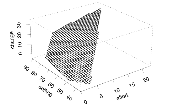
Figure 2.5 shows the estimated regression equation \( \hat{y} = \hat{\alpha} + \hat{\beta}_1 x_1 + \hat{\beta}_2 x_2 \) evaluated for a grid of values of the two predictors. The grid is confined to the range of the data on setting and effort. The regression plane may be viewed as an infinite set of regression lines. For any fixed value of setting, expected CBR decline is a linear function of effort with slope 0.97. For any fixed value of effort, expected CBR decline is a linear function of setting with slope 0.27.
It may be instructive to compare the results of the multiple regression analysis, which considered the two predictors simultaneously, with the results of the simple linear regression analyses, which considered the predictors one at a time.
The coefficients in a simple linear regression represent changes in the response that can be associated with a given predictor, and will be called gross effects. In our simple linear regression analysis of CBR decline as a function of family planning effort we found that, on the average, each additional point of family planning effort was associated with an additional 1.25 percentage point of CBR decline. Interpretation of gross effects must be cautious because comparisons involving one factor include, implicitly, other measured and unmeasured factors. In our example, when we compare countries with strong programs with countries with weak programs, we are also comparing implicitly countries with high and low social settings.
The coefficients in a multiple linear regression are more interesting because they represent changes in the response that can be associated with a given predictor for fixed values of other predictors, and will be called net effects. In our multiple regression analysis of CBR decline as a function of both family planning effort and social setting, we found that, on the average, each additional point of family planning effort was associated with an additional 0.97 percentage points of CBR decline if we held social setting constant, i.e. if we compared countries with the same social setting. Interpretation of this coefficient as measuring the effect of family planning effort is on somewhat firmer ground than for the gross effect, because the differences have been adjusted for social setting. Caution is in order, however, because there are bound to be other confounding factors that we have not taken into account.
In my view, the closest approximation we have to a true causal effect in social research based on observational data is a net effect in a multiple regression analysis that has controlled for all relevant factors, an ideal that may be approached but probably can never be attained. The alternative is a controlled experiment where units are assigned at random to various treatments, because the nature of the assignment itself guarantees that any ensuing differences, beyond those than can be attributed to chance, must be due to the treatment. In terms of our example, we are unable to randomize the allocation of countries to strong and weak programs. But we can use multiple regression as a tool to adjust the estimated effects for the confounding effects of observed covariates.
Table 2.6. Gross and Net Effects of Social Setting
and Family Planning Effort on CBR Decline
| Predictor | Effect | |
| Gross | Net | |
| Setting | 0.505 | 0.271 |
| Effort | 1.253 | 0.968 |
Gross and net effects may be presented in tabular form as shown in Table 2.6. In our example, the gross effect of family planning effort of 1.25 was reduced to 0.97 after adjustment for social setting, because part of the observed differences between countries with strong and weak programs could be attributed to the fact that the former tend to enjoy higher living standards. Similarly, the gross effect of social setting of 0.51 has been reduced to 0.27 after controlling for family planning effort, because part of the differences between richer and poorer countries could be attributed to the fact that the former tend to have stronger family planning programs.
Note, incidentally, that it is not reasonable to compare either gross or net effects across predictors, because the regression coefficients depend on the units of measurement. I could easily ‘increase’ the gross effect of family planning effort to 12.5 simply by dividing the scores by ten. One way to circumvent this problem is to standardize the response and all predictors, subtracting their means and dividing by their standard deviations. The regression coefficients for the standardized model (which are sometimes called ‘beta’ coefficients) are more directly comparable. This solution is particularly appealing when the variables do not have a natural unit of measurement, as is often the case for psychological test scores. On the other hand, standardized coefficients are heavily dependent on the range of the data; they should not be used, for example, if one has sampled high and low values of one predictor to increase efficiency, because that design would inflate the variance of the predictor and therefore reduce the standardized coefficient.
The basic principles of model comparison outlined earlier may be applied to multiple regression models. I will illustrate the procedures by considering a test for the significance of the entire regression, and a test for the significance of the net effect of one predictor after adjusting for the other.
Consider first the hypothesis that all coefficients other than the constant are zero, i.e.
\[ H_0: \beta_1 = \beta_2 = 0. \]To test the significance of the entire regression we start with the null model, which had a \( \mbox{RSS} \) of 2650.2 on 19 degrees of freedom. Adding the two linear predictors, social setting and family planning effort, reduces the \( \mbox{RSS} \) by 1956.2 at the expense of two d.f. Comparing this gain with the remaining \( \mbox{RSS} \) of 694.0 on 17 d.f. leads to an \( F \)-test of 24.0 on two and 17 d.f. This statistic is highly significant, with a P-value just above 0.00001. Thus, we have clear evidence that CBR decline is associated with social setting and family planning effort. Details of these calculations are shown in Table 2.7
Table 2.7. Analysis of Variance for Multiple Regression
of CBR Decline by Social Setting and Family Planning Effort
| Source of | Sum of | Degrees of | Mean | \(F\)- |
| variation | squares | freedom | squared | ratio |
| Regression | 1956.2 | 2 | 978.1 | 24.0 |
| Residual | 694.0 | 17 | 40.8 | |
| Total | 2650.2 | 19 |
In the above comparison we proceeded directly from the null model to the model with two predictors. A more detailed analysis is possible by adding the predictors one at a time. Recall from Section 2.4 that the model with social setting alone had a \( \mbox{RSS} \) of 1449.1 on 18 d.f., which represents a gain of 1201.1 over the null model. In turn, the multiple regression model with both social setting and family planning effort had a \( \mbox{RSS} \) of 694.0 on 17 d.f. which represents a gain of 755.1 over the model with social setting alone. These calculation are set out in the hierarchical anova shown in Table 2.8.
Table 2.8. Hierarchical Analysis of Variance for
Multiple Regression
of CBR Decline by Social Setting and Family Planning Effort
| Source of | Sum of | Degrees of | Mean | \(F\)- |
| variation | squares | freedom | squared | ratio |
| Setting | 1201.1 | 1 | 1201.1 | 29.4 |
| Effort\(|\)Setting | 755.1 | 1 | 755.1 | 18.5 |
| Residual | 694.0 | 17 | 40.8 | |
| Total | 2650.2 | 19 |
Note the following features of this table. First, adding the sums of squares and d.f.’s in the first two rows agrees with the results in the previous table; thus, we have further decomposed the sum of squares associated with the regression into a term attributed to social setting and a term added by family planning effort.
Second, the notation Effort\( | \)Setting emphasizes that we have considered first the contribution of setting and then the additional contribution of effort once setting is accounted for. The order we used seemed more natural for the problem at hand. An alternative decomposition would introduce effort first and then social setting. The corresponding hierarchical anova table is left as an exercise.
Third, the \( F \)-test for the additional contribution of family planning effort over and above social setting (which is \( F=18.5 \) from Table 2.8) coincides with the test for the coefficient of effort based on the estimate and its standard error (which is \( t=4.3 \) from Table 2.5), since \( 4.3^2 = 18.5 \). In both cases we are testing the hypothesis
\[ H_0: \beta_2=0 \]that the net effect of effort given setting is zero. Keep in mind that dividing estimates by standard errors tests the hypothesis that the variable in question has no effect after adjusting for all other variables. It is perfectly possible to find that two predictors are jointly significant while neither exceeds twice its standard error. This occurs when the predictors are highly correlated and either could account for (most of) the effects of the other.
A descriptive measure of how much we have advanced in our understanding of the response is given by the proportion of variance explained, which was first introduced in Section 2.4. In our case the two predictors have reduced the \( \mbox{RSS} \) from 2650.2 to 694.0, explaining 73.8%.
The square root of the proportion of variance explained is the multiple correlation coefficient, and measures the linear correlation between the response in one hand and all the predictors on the other. In our case \( R=0.859 \). This value can also be calculated directly as Pearson’s linear correlation between the response \( y \) and the fitted values \( \hat{y} \).
An alternative construction of \( R \) is of some interest. Suppose we want to measure the correlation between a single variable \( y \) and a set of variables (a vector) \( \boldsymbol{x} \). One approach reduces the problem to calculating Pearson’s \( r \) between two single variables, \( y \) and a linear combination \( z = {\mathbf c}'\boldsymbol{x} \) of the variables in \( \boldsymbol{x} \), and then taking the maximum over all possible vectors of coefficients c. Amazingly, the resulting maximum is \( R \) and the coefficients c are proportional to the estimated regression coefficients.
We can also calculate proportions of variance explained based on the hierarchical anova tables. Looking at Table 2.8, we note that setting explained 1201.1 of the total 2650.2, or 45.3%, while effort explained 755.1 of the same 2650.2, or 28.5%, for a total of 1956.2 out of 2650.2, or 73.8%. In a sense this calculation is not fair because setting is introduced before effort. An alternative calculation may focus on how much the second variable explains not out of the total, but out of the variation left unexplained by the first variable. In this light, effort explained 755.1 of the 1449.1 left unexplained by social setting, or 52.1%.
The square root of the proportion of variation explained by the second variable out of the amount left unexplained by the first is called the partial correlation coefficient, and measures the linear correlation between \( y \) and \( x_2 \) after adjusting for \( x_1 \). In our example, the linear correlation between CBR decline and effort after controlling for setting is 0.722.
The following calculation may be useful in interpreting this coefficient. First regress \( y \) on \( x_1 \) and calculate the residuals, or differences between observed and fitted values. Then regress \( x_2 \) on \( x_1 \) and calculate the residuals. Finally, calculate Pearson’s \( r \) between the two sets of residuals. The result is the partial correlation coefficient, which can thus be seen to measure the simple linear correlation between \( y \) and \( x_2 \) after removing the linear effects of \( x_1 \).
Partial correlation coefficients involving three variables can be calculated directly from the pairwise simple correlations. Let us index the response \( y \) as variable 0 and the predictors \( x_1 \) and \( x_2 \) as variables 1 and 2. Then the partial correlation between variables 0 and 2 adjusting for 1 is
\[ r_{02.1} = \frac { r_{02} - r_{01} r_{12} } { \sqrt{1-r_{01}^2} \sqrt{1-r_{12}^2} }, \]where \( r_{ij} \) denotes Pearson’s linear correlation between variables \( i \) and \( j \). The formulation given above is more general, because it can be used to compute the partial correlation between two variables (the response and one predictor) adjusting for any number of additional variables.
Table 2.9. Simple and Partial Correlations of CBR Decline
with Social Setting and Family Planning Effort
| Predictor | Correlation | |
| Simple | Partial | |
| Setting | 0.673 | 0.519 |
| Effort | 0.801 | 0.722 |
Simple and partial correlation coefficients can be compared in much the same vein as we compared gross and net effects earlier. Table 2.9 summarizes the simple and partial correlations between CBR decline on the one hand and social setting and family planning effort on the other. Note that the effect of effort is more pronounced and more resilient to adjustment than the effect of setting.
So far we have considered four models for the family planning effort data: the null model (\( \phi \)), the one-variate models involving either setting (\( x_1 \)) or effort (\( x_2 \)), and the additive model involving setting and effort (\( x_1+x_2 \)).
More complicated models may be obtained by considering higher order polynomial terms in either variable. Thus, we might consider adding the squares \( x_1^2 \) or \( x_2^2 \) to capture non-linearities in the effects of setting or effort. The squared terms are often highly correlated with the original variables, and on certain datasets this may cause numerical problems in estimation. A simple solution is to reduce the correlation by centering the variables before squaring them, using \( x_1 \) and \( (x_1-\bar{x}_1)^2 \) instead of \( x_1 \) and \( x_1^2 \). The correlation can be eliminated entirely, often in the context of designed experiments, by using orthogonal polynomials.
We could also consider adding the cross-product term \( x_1 x_2 \) to capture a form of interaction between setting and effort. In this model the linear predictor would be
\[\tag{2.17}\mu_i = \alpha + \beta_1 x_{i1} + \beta_2 x_{i2} + \beta_3 x_{i1} x_{i2}.\]This is simply a linear model where the model matrix \( \boldsymbol{X} \) has a column of ones for the constant, a column with the values of \( x_1 \), a column with the values of \( x_2 \), and a column with the products \( x_1 x_2 \). This is equivalent to creating a new variable, say \( x_3 \), which happens to be the product of the other two.
An important feature of this model is that the effect of any given variable now depends on the value of the other. To see this point consider fixing \( x_1 \) and viewing the expected response \( \mu \) as a function of \( x_2 \) for this fixed value of \( x_1 \). Rearranging terms in Equation 2.17 we find that \( \mu \) is a linear function of \( x_2 \):
\[ \mu_i = ( \alpha + \beta_1 x_{i1} ) + ( \beta_2 + \beta_3 x_{i1} ) x_{i2}, \]with both constant and slope depending on \( x_1 \). Specifically, the effect of \( x_2 \) on the response is itself a linear function of \( x_1 \); it starts from a baseline effect of \( \beta_2 \) when \( x_1 \) is zero, and has an additional effect of \( \beta_3 \) units for each unit increase in \( x_1 \).
The extensions considered here help emphasize a very important point about model building: the columns of the model matrix are not necessarily the predictors of interest, but can be any functions of them, including linear, quadratic or cross-product terms, or other transformations.
Are any of these refinements necessary for our example? To find out, fit the more elaborate models and see if you can obtain significant reductions of the residual sum of squares.