
We now consider what to do if the regression diagnostics discussed in the previous section indicate that the model is not adequate. The usual solutions involve transforming the response, transforming the predictors, or both.
The response is often transformed to achieve linearity and homoscedasticity or constant variance. Examples of variance stabilizing transformations are the square root, which tends to work well for counts, and the arc-sine transformation, which is often appropriate when the response is a proportion. These two solutions have fallen out of fashion as generalized linear models designed specifically to deal with counts and proportions have increased in popularity. My recommendation in these two cases is to abandon the linear model in favor of better alternatives such as Poisson regression and logistic regression.
Transformations to achieve linearity, or linearizing transformations, are still useful. The most popular of them is the logarithm, which is specially useful when one expects effects to be proportional to the response. To fix ideas consider a model with a single predictor \( x \), and suppose the response is expected to increase \( 100\rho \) percent for each point of increase in \( x \). Suppose further that the error term, denoted \( U \), is multiplicative. The model can then be written as
\[ Y = \gamma(1+\rho)^x U. \]Taking logs on both sides of the equation, we obtain a linear model for the transformed response
\[ \log Y = \alpha + \beta x + \epsilon, \]where the constant is \( \alpha = \log\gamma \), the slope is \( \beta=\log(1+\rho) \) and the error term is \( \epsilon=\log U \). The usual assumption of normal errors is equivalent to assuming that \( U \) has a log-normal distribution. In this example taking logs has transformed a relatively complicated multiplicative model to a familiar linear form.
This development shows, incidentally, how to interpret the slope in a linear regression model when the response is in the log scale. Solving for \( \rho \) in terms of \( \beta \), we see that a unit increase in \( x \) is associated with an increase of \( 100(e^\beta-1) \) percent in \( y \). If \( \beta \) is small, \( e^\beta-1 \approx \beta \), so the coefficient can be interpreted directly as a relative effect. For \( |\beta|<0.10 \) the absolute error of the approximation is less than 0.005 or half a percentage point. Thus, a coefficient of 0.10 can be interpreted as a 10% effect on the response.
A general problem with transformations is that the two aims of achieving linearity and constant variance may be in conflict. In generalized linear models the two aims are separated more clearly, as we will see later in the sequel.
Box and Cox (1964) have proposed a family of transformations that can be used with non-negative responses and which includes as special cases all the transformations in common use, including reciprocals, logarithms and square roots.
The basic idea is to work with the power transformation
\[ y^{(\lambda)} = \left\{ \begin{array}{ll} \frac{y^\lambda-1}{\lambda}& \lambda \ne 0 \ \log(y)& \lambda=0\ \end{array} \right. \]and assume that \( y^{(\lambda)} \) follows a normal linear model with parameters \( \boldsymbol{\beta} \) and \( \sigma^2 \) for some value of \( \lambda \). Note that this transformation is essentially \( y^\lambda \) for \( \lambda\ne0 \) and \( \log(y) \) for \( \lambda=0 \), but has been scaled to be continuous at \( \lambda=0 \). Useful values of \( \lambda \) are often found to be in the range \( (-2,2) \). Except for scaling factors, -1 is the reciprocal, 0 is the logarithm, 1/2 is the square root, 1 is the identity and 2 is the square.
Given a value of \( \lambda \), we can estimate the linear model parameters \( \boldsymbol{\beta} \) and \( \sigma^2 \) as usual, except that we work with the transformed response \( y^{(\lambda)} \) instead of \( y \). To select an appropriate transformation we need to try values of \( \lambda \) in a suitable range. Unfortunately, the resulting models cannot be compared in terms of their residual sums of squares because these are in different units. We therefore use a likelihood criterion.
Starting from the normal distribution of the transformed response \( y^{(\lambda)} \), we can change variables to obtain the distribution of \( y \). The resulting log-likelihood is
\[ \log L(\boldsymbol{\beta},\sigma^2,\lambda) = -\frac{n}{2}\log(2\pi\sigma^2) -\frac{1}{2}\sum(y_i^{(\lambda)}-\mu_i)^2/\sigma^2 +(\lambda-1)\sum \log(y_i), \]where the last term comes from the Jacobian of the transformation, which has derivative \( y^{\lambda-1} \) for all \( \lambda \). The other two terms are the usual normal likelihood, showing that we can estimate \( \boldsymbol{\beta} \) and \( \sigma^2 \) for any fixed value of \( \lambda \) by regressing the transformed response \( y^{(\lambda)} \) on the \( x \)’s. Substituting the m.l.e.’s of \( \boldsymbol{\beta} \) and \( \sigma^2 \) we obtain the concentrated or profile log-likelihood
\[ \log L(\lambda) = c - \frac{n}{2}\log\mbox{RSS}(y^{(\lambda)}) + (\lambda-1)\sum\log(y_i), \]where \( c = {\small \frac{n}{2}}\log(2\pi/n)- {\small \frac{n}{2}} \) is a constant not involving \( \lambda \).
Calculation of the profile log-likelihood can be simplified slightly by working with the alternative transformation
\[ z^{(\lambda)} = \left\{ \begin{array}{ll} \frac{y^{\lambda}-1}{\lambda \tilde{y}^{\lambda-1}}& \lambda\ne0\ \log(y) \tilde{y}& \lambda=0, \end{array} \right. \]where \( \tilde{y} \) is the geometric mean of the original response, best calculated as \( \tilde{y}=\exp(\sum\log(y_i)/n) \). The profile log-likelihood can then be written as
\[\tag{2.30}\log L(\lambda) = c - \frac{n}{2}\log\mbox{RSS}(z^{(\lambda)}),\]where \( \mbox{RSS}(z^{(\lambda)}) \) is the \( \mbox{RSS} \) after regressing \( z^{(\lambda)} \) on the \( x \)’s. Using this alternative transformation the models for different values of \( \lambda \) can be compared directly in terms of their \( \mbox{RSS} \)’s.
In practice we evaluate this profile log-likelihood for a range of possible values of \( \lambda \). Rather than selecting the exact maximum, one often rounds to a value such as \( -1 \), 0, 1/2, 1 or 2, particularly if the profile log-likelihood is relatively flat around the maximum.
More formally, let \( \hat{\lambda} \) denote the value that maximizes the profile likelihood. We can test the hypothesis \( H_0 \): \( \lambda=\lambda_0 \) for any fixed value \( \lambda_0 \) by calculating the likelihood ratio criterion
\[ \chi^2 = 2(\log L(\hat{\lambda}) - \log L(\lambda_0) ), \]which has approximately in large samples a chi-squared distribution with one d.f. We can also define a likelihood-based confidence interval for \( \lambda \) as the set of values that would be a accepted by the above test, i.e. the set of values for which twice the log-likelihood is within \( \chi^2_{1-\alpha,1} \) of twice the maximum log-likelihood. Identifying these values requires a numerical search procedure.
Box-Cox transformations are designed for non-negative responses, but can be applied to data that have occassional zero or negative values by adding a constant \( \alpha \) to the response before applying the power transformation. Although \( \alpha \) could be estimated, in practice one often uses a small value such as a half or one (depending, obviously, on the scale of the response).
Figure 2.9 Profile Log-likelihood for Box-Cox
Transformations
for Ancova Model of CBR
Decline by Setting and Effort
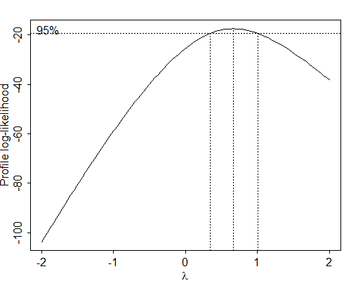
Let us apply this procedure to the program effort data. Since two countries show no decline in the CBR, we add 0.5 to all responses before transforming them. Figure 2.9 shows the profile log-likelihood as a function of \( \lambda \) for values in the range \( (-1,2) \). Note that \( \lambda=1 \) is not a bad choice, indicating that the model in the original scale is reasonable. A slightly better choice appears to be \( \lambda=0.5 \), which is equivalent to using \( \sqrt{y+0.5} \) as the response. Fitting this model leads to small changes in the significance of the coefficients of setting and strong programs, but does not materially alter any of the conclusions.
More formally, we note that the profile log-likelihood for \( \lambda=1 \) is \( -61.07 \). The maximum is attained at \( \lambda=0.67 \) and is \( -59.25 \). Twice the difference between these values gives a chi-squared statistic of \( 3.65 \) on one degree of freedom, which is below the 5% critical value of \( 3.84 \). Thus, there is no evidence that we need to transform the response. A more detailed search shows that a 95% confidence interval for \( \lambda \) goes from 0.34 to 1.01. The horizontal line in Figure 2.9, at a height of -61.17, identifies the limits of the likelihood-based confidence interval.
The Box-Cox procedure requires fitting a series of linear models, one for each trial value of \( \lambda \). Atkinson (1985) has proposed a simpler procedure that gives a quick indication of whether a transformation of the response is required at all. In practical terms, this technique involves adding to the model an auxiliary variable \( a \) defined as
\[\tag{2.31}a_i = y_i \: (\log(y_i/\tilde{y})-1),\]where \( \tilde{y} \) is the geometric mean of \( y \), as in the previous subsection. Let \( \gamma \) denote the coefficient of \( a \) in the expanded model. If the estimate of \( \gamma \) is significant, then a Box-Cox transformation is indicated. A preliminary estimate of the value of \( \lambda \) is \( 1-\hat{\gamma} \).
To see why this procedure works suppose the true model is
\[ \boldsymbol{z}^{(\lambda)} = \boldsymbol{X\beta} + \boldsymbol{\epsilon}, \]where we have used the scale-independent version of the Box-Cox transformation. Expanding the left-hand-side using a first-order Taylor series approximation around \( \lambda=1 \) gives
\[ z^{(\lambda)} \approx z^{(1)} + (\lambda-1) \left. \frac{d z^{(\lambda)}} {d\lambda} \right| _{\lambda=1}. \]The derivative evaluated at \( \lambda=1 \) is \( a+\log\tilde{y}+1 \), where \( a \) is given by Equation 2.31. The second term does not depend on \( \lambda \), so it can be absorbed into the constant. Note also that \( z^{(1)} = y-1 \). Using these results we can rewrite the model as
\[ \boldsymbol{y} \approx \boldsymbol{X\beta} + (1-\lambda)\boldsymbol{a} + \boldsymbol{\epsilon}. \]Thus, to a first-order approximation the coefficient of the ancillary variable is \( 1-\lambda \).
For the program effort data, adding the auxiliary variable \( a \) (calculated using CBR\( +1/2 \) to avoid taking the logarithm of zero) to the analysis of covariance model gives a coefficient of 0.59, suggesting a Box-Cox transformation with \( \lambda=0.41 \). This value is reasonably close to the square root transformation suggested by the profile log-likelihood. The associated \( t \)-statistic is significant at the two percent level, but the more precise likelihood ratio criterion of the previous section, though borderline, was not significant. In conclusion, we do not have strong evidence of a need to transform the response.
The Atkinson procedure is similar in spirit to a procedure first suggested by Box and Tidwell (1962) to check whether one of the predictors needs to be transformed. Specifically, to test whether one should use a transformation \( x^\lambda \) of a continuous predictor \( x \), these authors suggest adding the auxiliary covariate
\[ a_i = x_i \log(x_i) \]to a model that already has \( x \).
Let \( \hat{\gamma} \) denote the estimated coefficient of the auxiliary variate \( x\log(x) \) in the expanded model. This coefficient can be tested using the usual \( t \) statistic with \( n-p \) d.f. If the test is significant, it indicates a need to transform the predictor. A preliminary estimate of the appropriate transformation is given by \( \hat{\lambda}=\hat{\gamma}/\hat{\beta}+1 \), where \( \hat{\beta} \) is the estimated coefficient of \( x \) in the original model with \( x \) but not \( x\log(x) \).
We can apply this technique to the program effort data by calculating a new variable equal to the product of setting and its logarithm, and adding it to the covariance analysis model with setting and effort. The estimated coefficient is -0.030 with a standard error of 0.728, so there is no need to transform setting. Note, incidentally, that the effect of setting is not significant in this model.